Challenge

Project 2

SSadanand Shendolkar17 Mar 2023

POROJECT :-2

AIM:- The main goal of this project is to understand the functionality of a P1 hybrid and be able to model it.Honda Insight motor and battery are considered for this project.

Discription of P1 hybird model:-

The P1 architecture, with the electric motor is connected directly to the crankshaft, is the solution adopted by Honda on their first generation Integrated Motor Assist (IMA) technology. The electric motor functions as a generator, during vehicle deceleration, as an engine starter, and as a motor (to assist the engine) during vehicle accelerations. One of the biggest advantage of this solution is that the electric motor can provide higher torque than the BiSG, since there is no belt limitation (due to slip). However, since there is no speed / torque ratio between the electric machine and crankshaft, the torque requirements on the electric motor can be quite demanding.

Two examples of P1 MHEV architectures are:

Honda Insight Hybrid 2009 (with Integrated Motor Assist technology)
Mercedes Benz S400 Bluehybrid 2010

For example, the main characteristics of the P1 MHEV.

1] ELectric Machine Performance:-

Maximum torque up to 34 Nm.

Maximum power: 10KW

Efficiency: Up to 94 Percent

2] Advantages:-

Higher efficiency

The 12V starter can be removed

3] Disadvantages:-

Output torque limited by thje size of the elctric machine

Higher overall cost of the electrical components

Air cooling not possible for electric machine

Project initial step 1:-

Load the Project2 folder as the Current Folder in Matlab.

Run the “Project2_InitFile.m” Matlab script.

The Drive cycle selection is done here.

% Description:

%% Initialization File

% Initialization file for loading the variables for the Conventional vehicle simulation model

%% Vehicle Parameters

M = 1500; % Vehicle weight [kg]

Cr = 0.015; % Rolling resistance coefficient

Rw = 0.35; % Rolling radius [m]

Cd = 0.33; % Drag coefficient

Af = 2; % Frontal area [m2]

rhoa = 1.225; % Air density [kg/m3]

Vwind = 0; % Wind velocity [kmph]

g = 9.81; % Gravitational acceleration [m/s2]

theta = 0; % Slope [deg]

myu_road_tire = 1; % Coefficient of friction between tire - road interface

%% Powertrain Parameters

FDR = 3.73; % Final Drive Ratio / Diff Ratio

DiffEff = 0.99; % Differential efficiency (assumed independent of operating conditions)

NumGear = 4; % Number of gears in transmission

TransGear = [1:NumGear]; % Transmission Gears

TransRatio = [3.06, 1.62, 1, 0.7]; % Corresponding Transmission ratios

TransEff = 0.90; % Transmission efficiency (assumed independent of operating conditions)

TC_SR = [0, .5, .6, .7, .8, .87, .92, .94, .96, .97, 1]; % Torque Converter Speed Ratio (Matlab default) -> TurbSpd/PumpSpd

TC_TR = [2.232, 1.5462, 1.4058, 1.2746, 1.1528, 1.0732, 1.0192, 1, 1, 1, 1]; % Torque Converter Torque Ratio (Matlab default) -> TurbTrq/PumpTrq

TC_Cf = 1e-4 * [.72558, .66322, .63463, .59042, .51331, .4144, .29287, .22444, .12186, .04386, 0]; % Torque Converter Capacity Factor (Matlab default) -> PumpTrq/PumpSpd^2 [Nm/rpm^2]

load Vehicle_Data/Engine_data_1_9L_Saturn_95kW

load Vehicle_Data/Trans_Shift_map

load Vehicle_Data/EM_Honda_Insight_10kW

load Vehicle_Data/ESS_NiMH6

ESS_init_soc = 0.8;

ESS_soc_max = 0.9;

ESS_soc_min = 0.6;

%% Driver Parameters

Kp = 10; % P gain for driver PI model

Ki = 1; % I gain for driver PI model

Drive_Cycle_Select = 1; % Drive cycle selection

% Drive cycle values in m/s

if Drive_Cycle_Select == 1

load DriveCycles/UDDS;

elseif Drive_Cycle_Select == 2

load DriveCycles/HWFET;

elseif Drive_Cycle_Select == 3

load DriveCycles/FTP;

elseif Drive_Cycle_Select == 4

load DriveCycles/US06;

elseif Drive_Cycle_Select == 5

load DriveCycles/NEDC;

elseif Drive_Cycle_Select == 6

load DriveCycles/WLTP;

end

time_end = cyc_time(end);

vel_end = cyc_vel(end);

After run this coding file open simulink model.

Vehicle Model:-

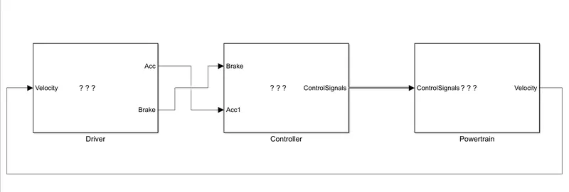
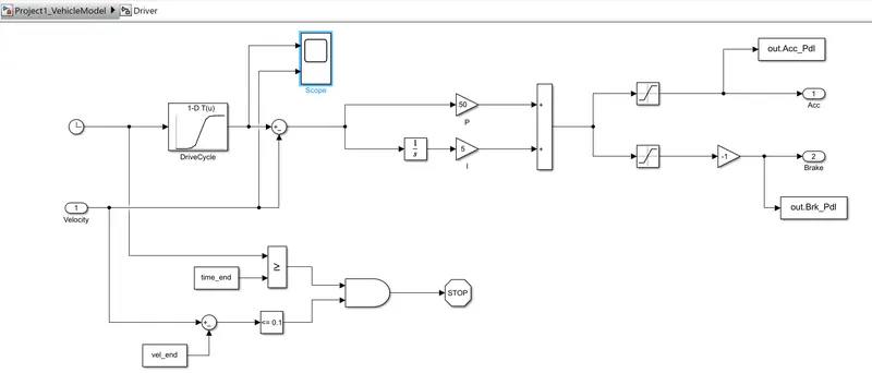
2) Driver Model :- In this model using a ‘Driver’ block, which is a basic PI controller that generates accelerator and brake pedal outputs to match the desired and actual vehicle speeds.

3) Controller :-The Controller block is the brains of the vehicle, representing the electronic controls units. It is based on the driver inputs, it generates desired engine torque, desired transmission gear desired motor torque and desired brake torque.

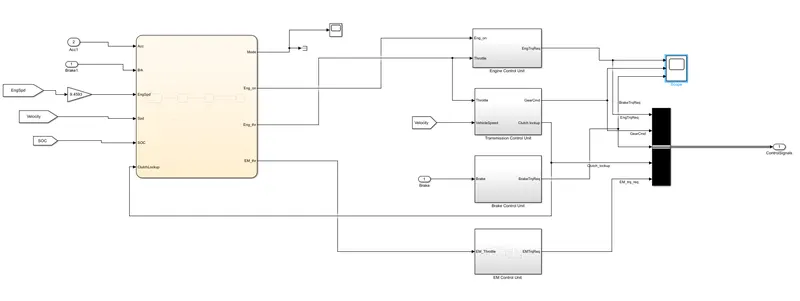
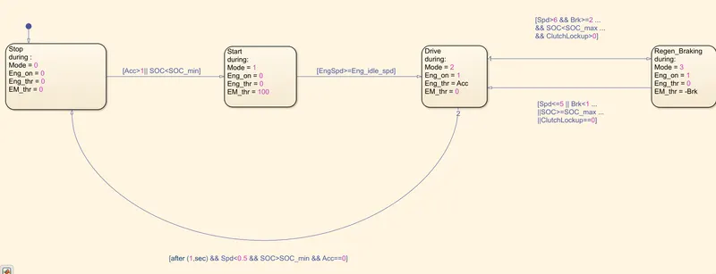
Chart :-In this we created four conditions as stop, start, drive and regenration braking. The initial block represent the stop condition. In which the engine is off.Then the second block represent start condition.third block ie. engine is on and the engine throttle is also having positive value from the driver but the electric motor throttle is zero.

In fourth case represents regenrative braking which is model 3 In this state the engine is on but the engine throttle is having no input from driver whereas the electric moto receives the negative power due to braking.

The inputs are given to chart is Acceleration, barke, engine speed, vehicle speed, SOC, and clutch lockup.

The output we get from the chart is mode, engine condition, engine throttle condition, and electric motor throttle condition

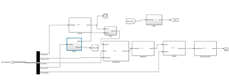
Powertrain:-

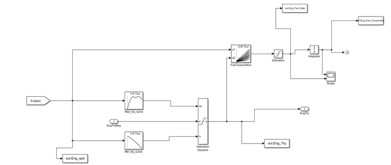
Engine:-

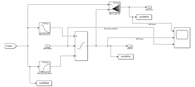
Electric motor :-

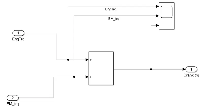
Crnak:-

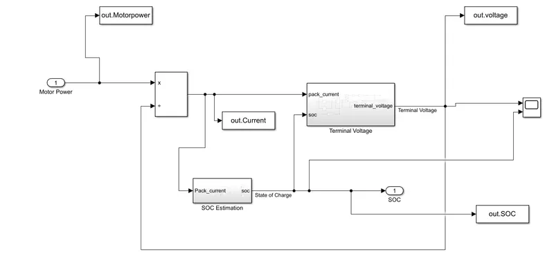
ESS(battery ):-n this we give input as power then it multiply and give to pack current. then from soc estimation meet output SOC its give to terminal voltage as input and then meet terminal voltage as output.

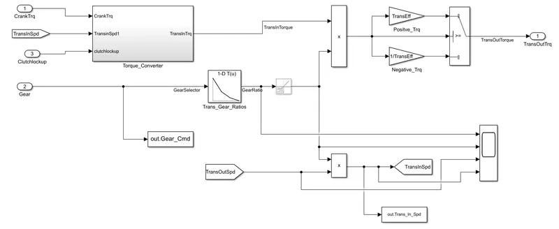
Transmission :-

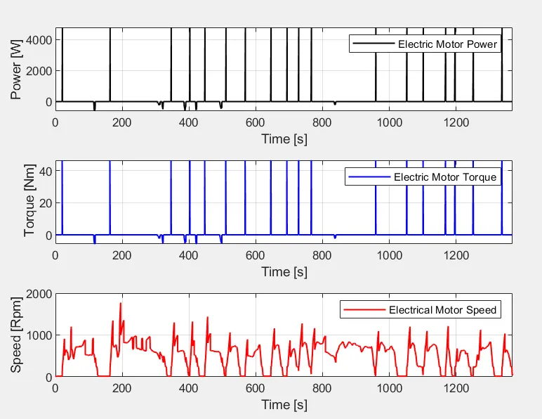
3)step -3 After running simulink model .Now post processing file is build up and run for getting results for different cycle .

Post processing file

%% Renaming variables

Time = out.tout;

Acc_Pdl = out.Acc_Pdl; % Accelerator pedal [%]

Brk_Pdl = out.Brk_Pdl; % Brake pedal [%]

Gear_Cmd = out.Gear_Cmd; % Transmission gear

Trans_In_Spd = out.Trans_In_Spd*30/pi; % Transmission input speed [rpm]

Trans_Out_Spd = out.Trans_Out_Spd*30/pi;% Transmission output speed [rpm]

Eng_Trq = out.Eng_Trq; % Engine brake torque [Nm]

Eng_Spd = out.Eng_spd*30/pi; % Engine speed [rpm]

Eng_Fuel_Consump = out.Eng_Fuel_Consumption; % Engine fuel consumption [g]

Veh_Dist = out.Veh_Dist/1000; % Distance traveled by vehicle [km]

Veh_Spd = out.Veh_Spd*18/5; % Vehicle speed [kmph]

Wheel_Speed = out.WheelSpd; % Wheel speed [kmph]

Eng_Fuel_Rate = out.Eng_Fuel_Rate % Engine fuel rate [%]

EM_Speed = out.EMSpd*18/5; % Electric Motor Speed

EM_Power = out.EMPwr; % Electric Motor Power

EM_Torque = out.EMTrq; % Electric Motor Torque

Term_Volt = out.voltage; % Terminal Voltage of battery

Soc = out.SOC; % State Of Charge

Pack_Current = out.Current; %Pack current of battery

%% Data Analysis

Eng_Pwr = Eng_Spd.*pi./30.*Eng_Trq./1000; % Engine brake power [kW]

rho_petrol = 0.7197; % Density of petrol [kg/L]

kmpl = Veh_Dist(end)/(Eng_Fuel_Consump(end)/1000/rho_petrol) % Fuel economy [kmpl]

figure(1)

hold on

grid on

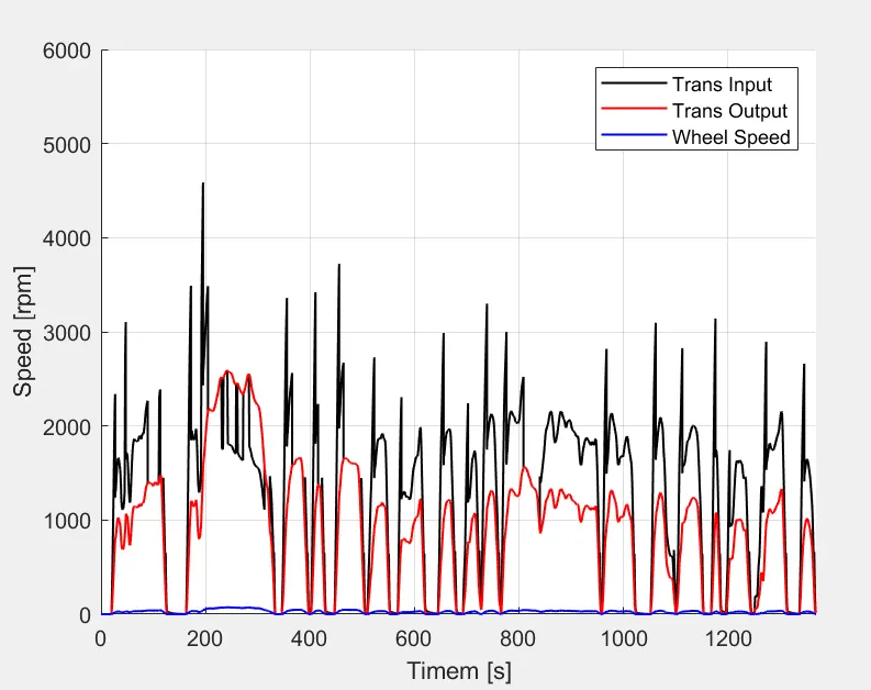
plot(Time, Trans_In_Spd, 'linewidth', 1, 'Color', 'black');

plot(Time, Trans_Out_Spd, 'linewidth', 1, 'Color', 'red');

plot(Time, Wheel_Speed, 'linewidth',1, 'color', 'blue')

ylabel('Speed [rpm]')

xlabel('Timem [s]')

xlim([0, Time(end)]);

ylim([0, 6000]);

legend('Trans Input','Trans Output','Wheel Speed');

%% Plotting Engine speed, Engine Torque, Engine Power,Engine fuel rate,Engine fuel consumption wrt Time

figure(2)

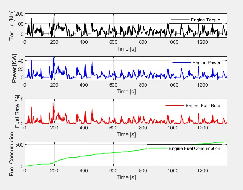
subplot(4,1,1)

plot(Time,Eng_Trq,'linewidth',1,'color','black')

xlim([0, Time(end)]);

xlabel('Time [s]')

ylabel('Torque [Nm]')

legend('Engine Torque')

grid on

subplot(4,1,2)

plot(Time,Eng_Pwr,'linewidth',1,'color','blue')

xlim([0, Time(end)]);

xlabel('Time [s]')

ylabel('Power [KW]')

legend('Engine Power')

grid on

subplot(4,1,3)

plot(Time,Eng_Fuel_Rate,'linewidth',1,'color','red')

xlim([0, Time(end)]);

xlabel('Time [s]')

ylabel('Fuel Rate [%]')

legend('Engine Fuel Rate')

grid on

subplot(4,1,4)

plot(Time,Eng_Fuel_Consump,'linewidth',1,'color','green')

xlim([0, Time(end)]);

xlabel('Time [s]')

ylabel('Fuel Consumption')

legend('Engine Fuel Consumption')

grid on

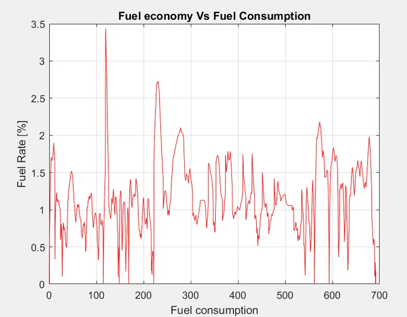
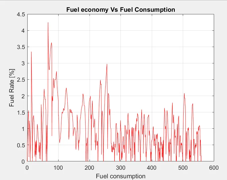
% Plotting fuel economy Vs Engine Fuel consumption

figure(3)

plot(Eng_Fuel_Consump,Eng_Fuel_Rate,'color','r')

xlabel('Fuel consumption')

ylabel('Fuel Rate [%]')

title('Fuel economy Vs Fuel Consumption')

grid on

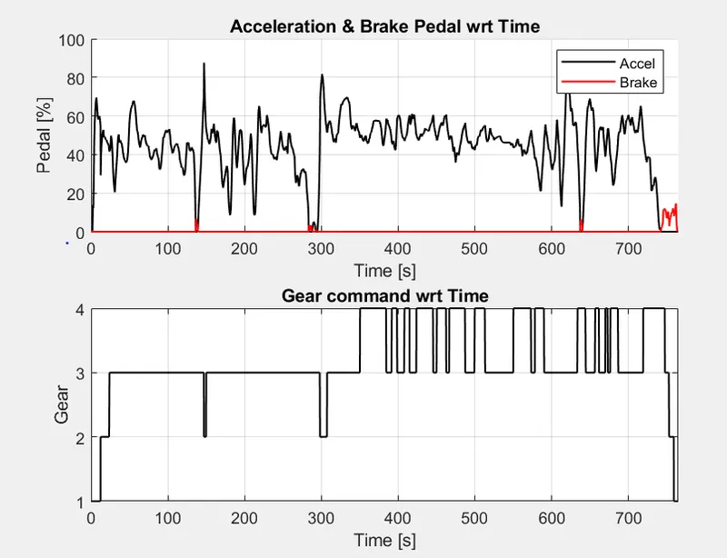
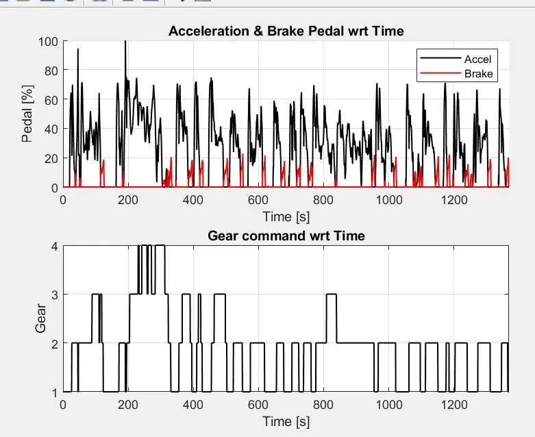
%% Potting Accelerator pedal, Brake pedal and gear command with respect to time

figure(4)

subplot(2,1,1)

hold on

plot(Time, Acc_Pdl, 'linewidth', 1, 'Color', 'black');

plot(Time, Brk_Pdl, 'linewidth', 1, 'Color', 'red');

ylabel('Pedal [%]')

xlabel('Time [s]');

xlim([0, Time(end)]);

grid on

legend('Accel','Brake');

title('Acceleration & Brake Pedal wrt Time')

subplot(2,1,2)

plot(Time, Gear_Cmd, 'linewidth', 1, 'Color', 'black');

xlim([0, Time(end)]);

xlabel('Time [s]');

ylabel('Gear');

grid on

title('Gear command wrt Time')

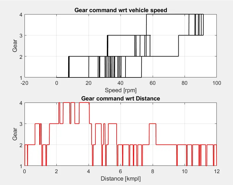
% Plotting gear command vehicle desired with actual speed

figure(5)

subplot(2,1,1)

plot(Veh_Spd, Gear_Cmd, 'linewidth', 1, 'Color', 'black');

xlabel('Speed [rpm]');

ylabel('Gear');

grid on

title('Gear command wrt vehicle speed')

subplot(2,1,2)

plot(Veh_Dist, Gear_Cmd, 'linewidth', 1, 'Color', 'red');

xlabel('Distance [kmpl]');

ylabel('Gear');

grid on

title('Gear command wrt Distance')

%% Plotting engine operating points on engine fuel map

figure('Name','Engine Operating Points');

hold on

grid on

title('Engine Operating Points','fontsize',12);

p1=plot(Eng_map_spd*30/pi,Eng_max_trq,'linewidth',2,'color','r');

p2=line([Eng_map_spd(end)*30/pi Eng_map_spd(end)*30/pi],[0 Eng_max_trq(end)]);

set(p2,'linewidth',1,'linestyle','--','color','k');

p3=line([Eng_map_spd(1)*30/pi Eng_map_spd(1)*30/pi],[0 Eng_max_trq(1)]);

set(p3,'linewidth',1,'linestyle','--','color','k');

[c,h] = contour(Eng_map_spd'*30/pi,Eng_map_trq,Eng_fuel_map');

clabel(c,h);

xlabel('Engine Speed [rpm]');

ylabel('Engine Torque [Nm]');

title('Engine Fuel Consumption Map [g/s]');

legend([p1 p3],{'Max Curve','Operating Points'});

axis([Eng_map_spd(1)*30/pi Eng_map_spd(end)*30/pi 0 Eng_map_trq(end)]);

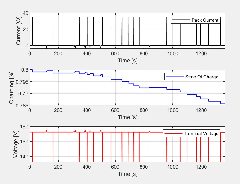
%% State of Charge, Pack Current, And Terminal Voltage with respect to Time

figure(6)

subplot(3,1,1)

plot(Time,Pack_Current,'linewidth',1,'color','black')

xlim([0, Time(end)]);

xlabel('Time [s]')

ylabel('Current [W]')

legend('Pack Current')

grid on

subplot(3,1,2)

plot(Time,Soc,'linewidth',1,'color','blue')

xlim([0, Time(end)]);

xlabel('Time [s]')

ylabel('Charging [%]')

legend('State Of Charge')

grid on

subplot(3,1,3)

plot(Time,Term_Volt,'linewidth',1,'color','red')

xlim([0, Time(end)]);

xlabel('Time [s]')

ylabel('Voltage [V]')

legend('Terminal Voltage')

grid on

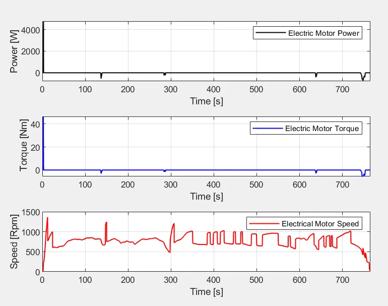
%% Motor Speed, Torque, Motor input power with respect to Time

figure(7)

subplot(3,1,1)

plot(Time,EM_Power,'linewidth',1,'color','black')

xlim([0, Time(end)]);

xlabel('Time [s]')

ylabel('Power [W]')

legend('Electric Motor Power ')

grid on

subplot(3,1,2)

plot(Time,EM_Torque,'linewidth',1,'color','blue')

xlim([0, Time(end)]);

xlabel('Time [s]')

ylabel(' Torque [Nm]')

legend('Electric Motor Torque')

grid on

subplot(3,1,3)

plot(Time,EM_Speed,'linewidth',1,'color','red')

xlim([0, Time(end)]);

xlabel('Time [s]')

ylabel('Speed [Rpm]')

legend('Electrical Motor Speed')

grid on

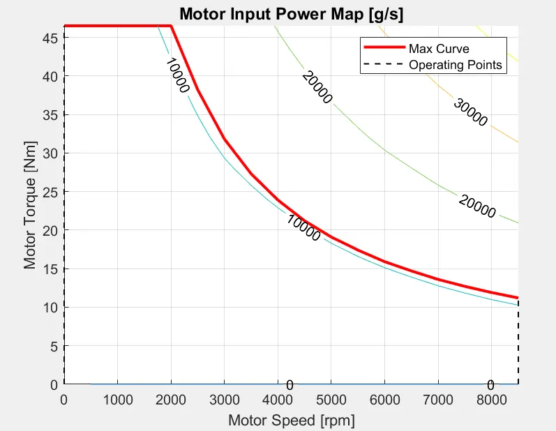
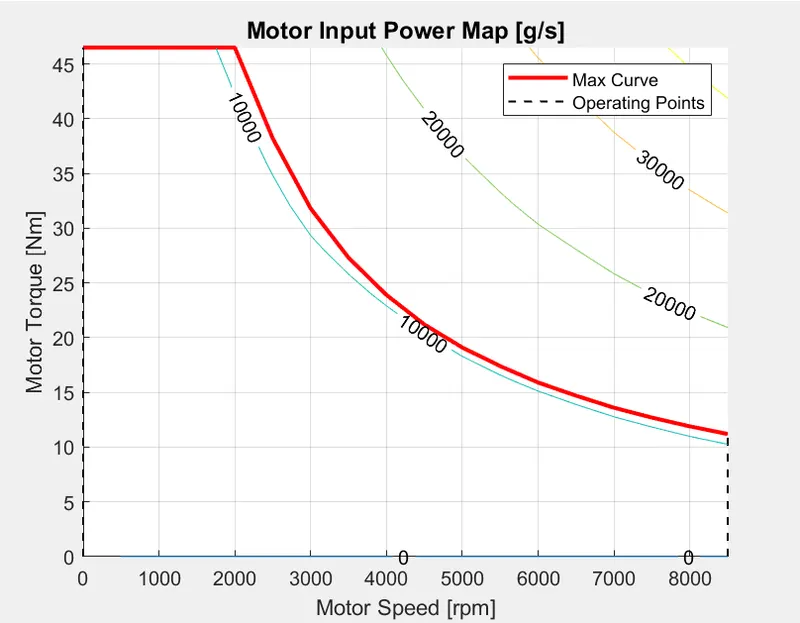
%% Plotting EM Operating Points on motor input power Map

figure('Name','Electric Motor Operating Points');

hold on

grid on

title('Electric Motor Operating Points','fontsize',12);

p1=plot(EM_map_spd*30/pi,EM_max_trq,'linewidth',2,'color','r');

p2=line([EM_map_spd(end)*30/pi EM_map_spd(end)*30/pi],[0 EM_max_trq(end)]);

set(p2,'linewidth',1,'linestyle','--','color','k');

p3=line([EM_map_spd(1)*30/pi EM_map_spd(1)*30/pi],[0 EM_max_trq(1)]);

set(p3,'linewidth',1,'linestyle','--','color','k');

[c,h] = contour(EM_map_spd'*30/pi,EM_map_trq,EM_inpwr_map');

clabel(c,h);

xlabel('Motor Speed [rpm]');

ylabel('Motor Torque [Nm]');

title('Motor Input Power Map [g/s]');

legend([p1 p3],{'Max Curve','Operating Points'});

axis([EM_map_spd(1)*30/pi EM_map_spd(end)*30/pi 0 EM_map_trq(end)]);

Results and Plots :-

1)HWFET (Highway ) drive cycle :

S.No	Drive cycle	Fuel Economy Number (KMpl)
1	UDDS	15.0773
2	HWFET	17.16

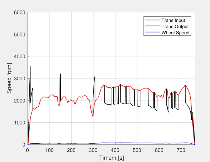
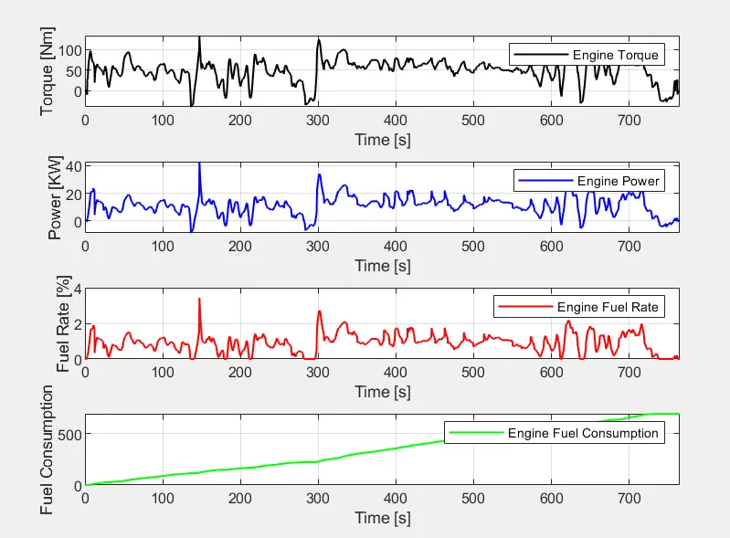
From the results it is proved that fuel economy of HWFET is high compared to UDDS. It is because in urban driving the vehicle encounters more traffic and it has to stop for fever distance and it consumes more fuel at the starting. In HWFET the vehicle have not traffic and it moves without use of too much braking so it will have more fuel economy number.

S.No	Drive cycle	Fuel Economy Number (KMpl)
1	UDDS	14.2
2	HWFET	16.5

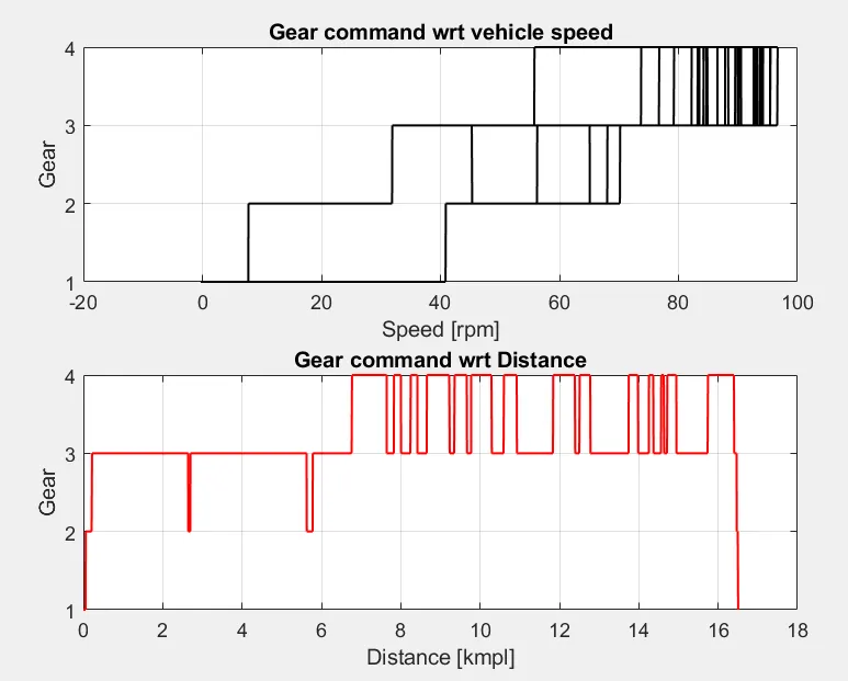
From the result fuel economy numbers for project 2 is higher when compared to project 1 because of implementing the electric motor as it is P1 hybrid it may not have much variation in the fuel economy but as we implement other architechture it will increase by huge amount.

2)For UDDS(Urbon drive ):

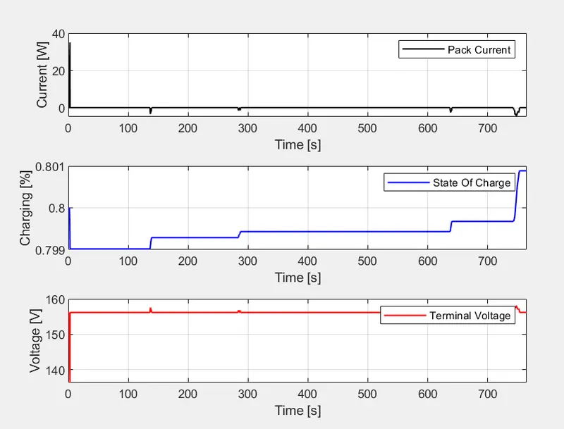
The pack voltage and current will have more fluctuations in UDDS as compared to HWFET cycle because of the frequent start and stops throughout the drive and the battery has to provide the energgy everytime when the car is starting from the idle position.
SOC decreased in the UDDS cycle wrt time but it has increased in HWFET cycle.
Therewill be more fluctuations in UDDS cycle compared to HWFET cycle because UDDS has many starts and stops due to traffic as the purpose of motor in P! hybrid is initiation of crank rotation and they are more in UDDS cycle when compared to HWFET cycle

Conclusion:-

Performance UDDS drive cycle and HWFET drive cycle are analysed and the graphs are plotted

Time trace for engine, Transmission input, Transmission output and wheelspeed with respect to time.
Engine torque, Engine power, Fuel rate and Fuel consumption with respect to time.
Accelerator and brake pedal, gear command and vehicle desired, actual speed, vehicle distance with respect to time.
Engine operating points on the engine fuel map with respect to time.

Project 2

Ship work like this
in your own course.

Talk to a career counsellor

Ship work like thisin your own course.

Talk to a career counsellor

Ship work like this
in your own course.