Simulink - System-level simulation of an All-Terrain Vehicle (CVT)

System-level simulation of an All-Terrain Vehicle

Aim:

• To study and analyse the BAJA All Terrain Vehicle (ATV) model using Simulink.

Program used:

• Software - Simulink (simscape) - Version 2020a.

Objectives:

• To prepare a technical report of ATV model with and without Lookup table.

Theory:

• All Terrain Vehicle:
  • An all-terrain vehicle (ATV), also known as a quad bike, or simply a quad.It is a vehicle that travels on low-pressure tires, with a seat that is straddled by the operator, along with handlebars for steering control. ATVs are intended for use by a single operator, although some companies have developed ATVs intended for use by the operator and one passenger.
• SAE BAJA ATV:
  • Baja SAE is an intercollegiate engineering design competition for undergraduate and graduate engineering students. The object of the competition is to simulate real-world engineering design projects and their related challenges.
  • These vehicles need to go through 2 types of events, Static Events and Dynamic Events.
  • Static Events:
    • Technical Inspection
    • Cost Event
    • Design Judging
    • Sales Presentation
  • Dynamic Events:
    • Acceleration
    • Hill Climb or Traction Event and Maneuverability
    • Specialty Events
    • Endurance Race
• CVT (Continuously Variable Transmission) :
  • A Continuously Variable Transmission is an automatic transmission and it is a type of single-speed automatic gearbox. that can change seamlessly through a continuous range of gear ratios. when compared to other transmissions that provide a limited number of gear ratios in fixed steps. The flexibility of a CVT with suitable control may allow the engine to operate at a constant RPM while the vehicle moves at varying speeds.

Major Components used:

• Generic Engine Block:
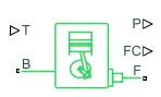
  • The Generic Engine block represents a general internal combustion engine. Engine types include spark-ignition and diesel. Speed-power and speed-torque parameterizations are provided. A throttle physical signal input specifies the normalized engine torque. Optional dynamic parameters include crankshaft inertia and response time lag. A physical signal port outputs engine fuel consumption rate based on choice of fuel consumption model. Optional speed and redline controllers prevent engine stall and enable cruise control.
  • 
  • Block Ports:

    • B	Rotational conserving port representing the engine block
      F	Rotational Conserving port representing the engine crankshaft
      T	Physical signal input port specifying the normalized engine throttle level
      P	Physical signal output port reporting the instantaneous engine power, in W
      FC	Physical signal output port reporting the fuel consumption rate, in kg/s

• Variable Ratio Transmission Block:
  • The Variable Ratio Transmission block represents a gearbox that dynamically transfers motion and torque between the two connected driveshaft axes, base and follower. Variable Ratio Transmission is a dynamical mechanism for transferring motion and torque between base and follower. If the relative compliance ϕ between the axes is absent, the block is equivalent to a gear with a variable ratio g_FB(t). Such a gear imposes a time-dependent kinematic constraint on the motions of the two driveshafts
  • 
  • Block Ports:
    

    • B and F are rotational conserving ports representing, respectively, the base and follower driveshafts.

    • Variable gear ratio g_FB(t) can be specified as a function of time at the physical signal input at port r. If the signal value becomes zero or negative, the simulation stops with an error.

• Simple Gear:
  • The Simple Gear block represents a gearbox that constrains the connected driveline axes of the base gear, B, and the follower gear, F, to corotate with a fixed ratio that you specify. You choose whether the follower axis rotates in the same or opposite direction as the base axis. If they rotate in the same direction, the angular velocity of the follower, ω_F, and the angular velocity of the base, ω_B, have the same sign. If they rotate in opposite directions, ω_F and ω_B have opposite signs.
  • Gear ratio: `g_{FB} = r_F/r_B = N_F/N_B`

    • r_F is the radius of the follower gear.

    • ω_F is the angular velocity of the follower gear.

    • r_B is the radius of the base gear.

    • ω_B is the angular velocity of the base gear.

  • 
    • Block Ports:
      • B indicates Base
      • F indicates Follower
• Vehicle Body:

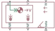
  • The Vehicle Body block represents a two-axle vehicle body in longitudinal motion. The vehicle can have the same or a different number of wheels on each axle. For example, two wheels on the front axle and one wheel on the rear axle. The vehicle wheels are assumed identical in size. The vehicle can also have a center of gravity (CG) that is at or below the plane of travel.

  • 
  • Block Ports:
    • Inputs:
      • W - Headwind speed, m/s
      • beta - Road incline angle,rad
      • CG - Center of gravity,m
      • M - Mass,kg
      • J - External moment of inertia, kg*m^2
    • Outputs:
      • V - Longitudnal velocity,m/s
      • NF - Front axle normal force,N
      • NR - Rear axle normal force,N
    • Conserving:
      • H - Horizontal motion
• Tire:
  • The Tire block models a tire with longitudinal behavior given by the Magic Formula, an empirical equation based on four fitting coefficients. The block can model tire dynamics under constant or variable pavement conditions.
  • 
  • Block Ports:
    • Inputs:
      • N - Normal force
      • M - magic formula coefficients
    • Outputs:
      • S - slip
    • Conserving
      • A - Axle
      • H - Hub
• Double-Shoe Brake:
  • The Double-Shoe Brake block represents a frictional brake with two pivoted rigid shoes that press against a rotating drum to produce a braking action. The rigid shoes sit inside or outside the rotating drum in a diametrically opposed configuration. A positive actuating force causes the rigid shoes to press against the rotating drum. Viscous and contact friction between the drum and the rigid shoe surfaces cause the rotating drum to decelerate.
  • 
  • Ports:
    • F - Actuating force
    • S - Drum shaft rotation
    • H - Heat flow

Types of models:

1. CVT model
2. CVT model dashboard
3. CVT model data
4. CVT model mapped
5. CVT model mapped dashboard

#1 Model: CVT model

Models and Subsystems

• Main Model:
• 
• Engine sensor:
• 
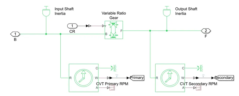
• CVT Subsystem:
• 
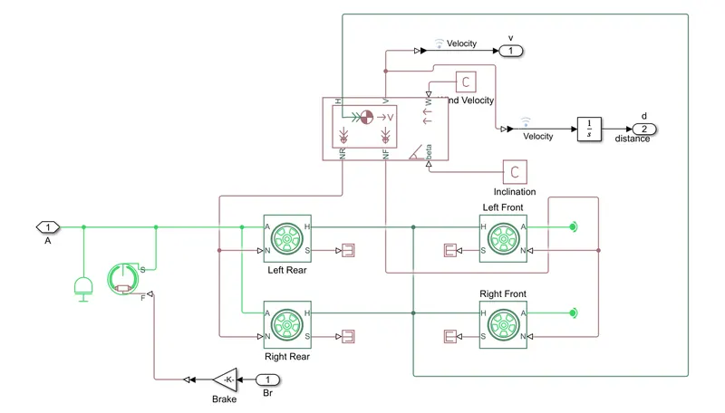
• Vehicle Body Subsystem:
• 

Flow Process:

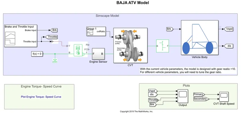
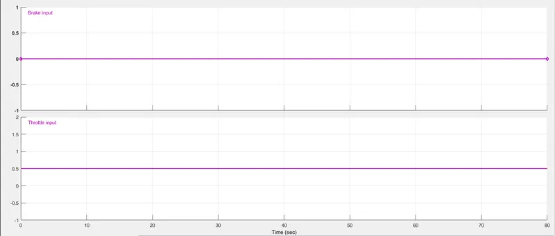
1. The inital input of the system are 'Throttle Input' and 'Brake Input'. These inputs are given by using signal builder and only throttle signal is given as input to the generic engine block
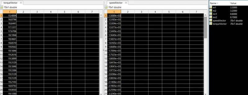
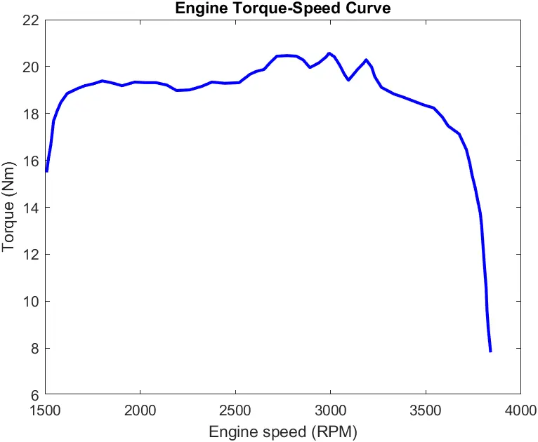
2. For the generic engine block the parameters are given by using 'Tabulated torque data', the speed vector and torque vector are given as input using matlab workspace.
3. The initial RPM of the engine block is givne as 1750RPM. So, the initial throttle should be 0.5 to initiate the simulation.
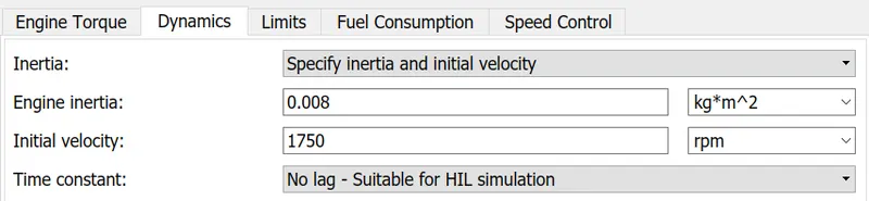
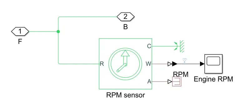
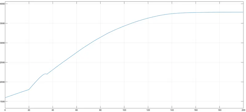
4. The output form the engine block which is required is RPM of crank shaft, this is connected to the engine sensor subsystem, which consists of Ideal rotational motion sensor. This sensor helps to plot 'Engine RPM'. This RPM is given as input to the CVT subsystem.
5. In this model CVT ratio varies with time.So, a signal builder is used to give the input to the block.
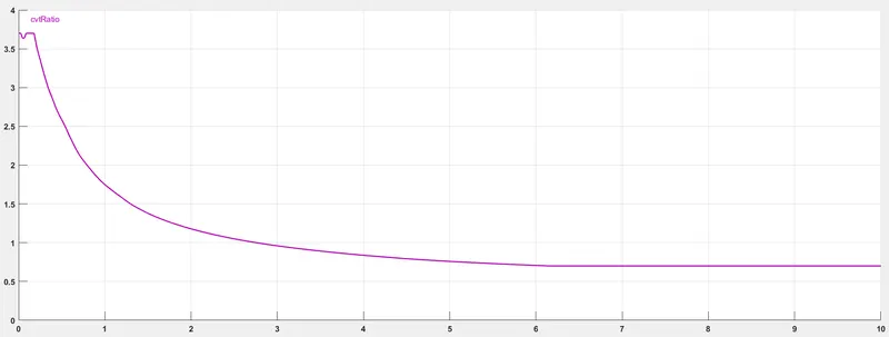
6. Two rotational sensors are used to log the RPM data of both primary and secondary pulleys.
7. The output of the secondary pulley is given to a 'simple gear' which has a fixed gear ratio. The output form this block is given as the input RPM to the Tire block in Vehicle body subsystem.
8. In the vehicle body subsystem, vehicle parameters are given using vehicle body block. The outputs from this block are Normal forces both front and rear, velocity of the vehicle.
9. In the main model space, these values are plotted using scopes and goto, from blocks.

Output Plots:

1. Engine Torque vs RPM curve: 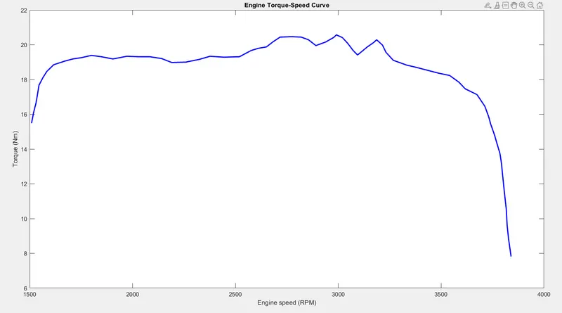This plot shows the input parameters which are given to the Generic Engine Block as Torque vector and Speed Vector
2. Velocity, Distance, Throttle and Brake vs time 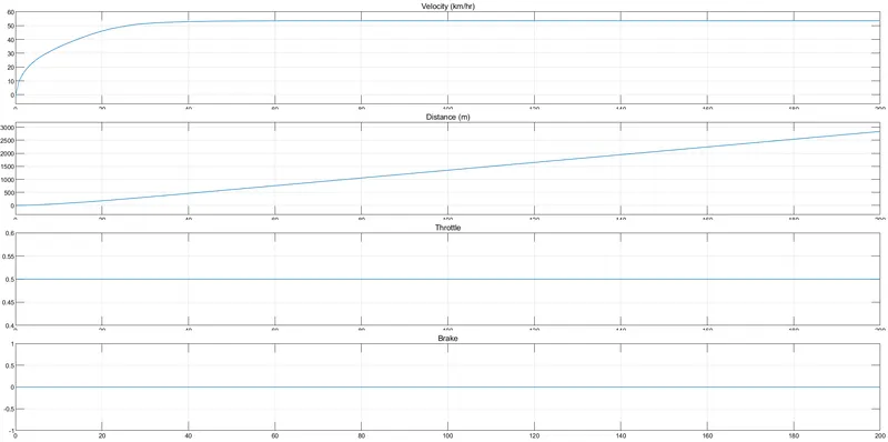This plot show variation in velocity with respect to time. After a certain time the plot is a straight line which is true because the gear ratio is constant after some time and the throttle is maintained at 0.5. The distance covered is increasing with repect to time as the vehicle did not stop. The conversion of velocity is done in PS-simulink converter.
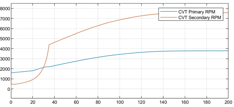
3. CVT Primary and Secondary RPM vs Time 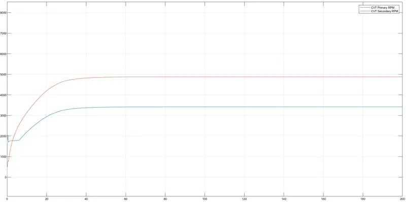As the CVT gear ratio is decresing from a high value to a low value. In the initial time of simulation the RPM, Gear ratio is Greater than 1 so RPM of secondary is less than primary and as the simulation is carried out for a longer time the secondary pulley RPM is more than primary which indicates the gear ratio in CVT is less than 1.

#2 Model: CVT model with Dashboard:

Models and Subsystems

• Main Model:
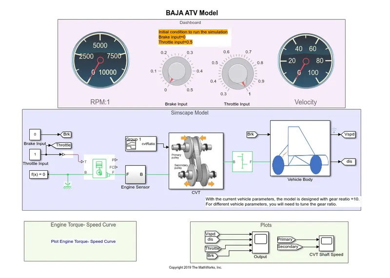
• SubSystems:
  • All the subsystems are same as '#1 Model: CVT model'

Flow Process:

• The Flow process is same as '#1 Model: CVT model'.But the throttle input and brake input are given using user controlled knobs.

Output Plots:

1. Engine Torque vs RPM curve: This plot shows the input parameters which are given to the Generic Engine Block as Torque vector and Speed Vector
2. Velocity, Distance, Throttle and Brake vs time 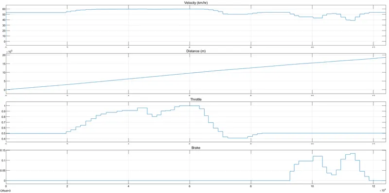This plot show variation in velocity with respect to time. As the throttle and brake input are user defined by using knobs, there are steps created.
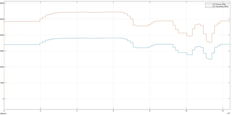
3. CVT Primary and Secondary RPM vs Time

#3 Model CVT model data

Models and Subsystems:

• Main Model:
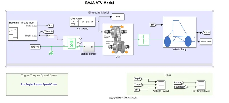
• Subsystems: All the subsystems are same as '#1 Model: CVT model'

Flow Process:

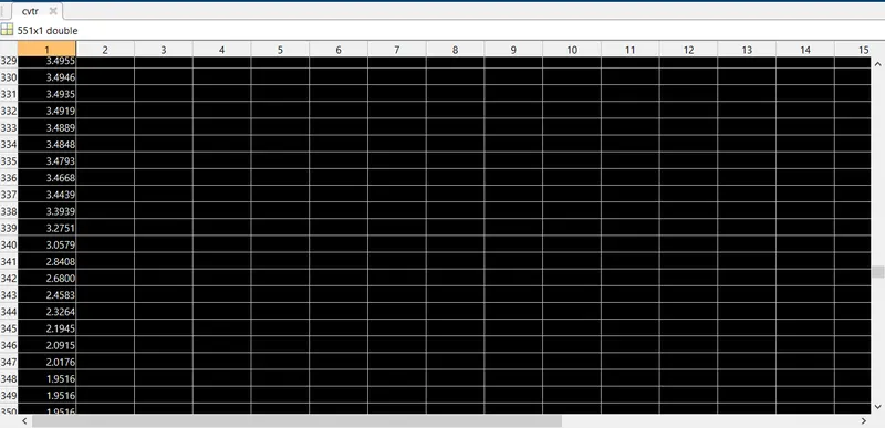
• The flow process is also similar to that of '#1Model: CVT model'. But there is an extra block added called 'To workspace' which is connected to the CVT gear ratio. This block is used to send the CVT ratio to the Matlab workspace and can be used for further analysis.

Output:

• The output plots are same as the '#1 Model: CVT model'.
• cvtr in matlab workspace:

#4 Model CVT model mapped

Model and Subsystems:

• Model:
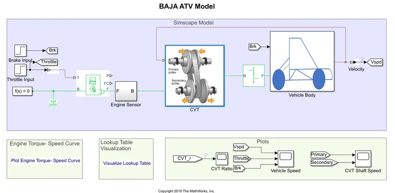
• Subsystems: All the subsystems are same as '#1 Model: CVT model'

Flow Process:

1. The flow process is similar to that of '#1 Model: CVT model'
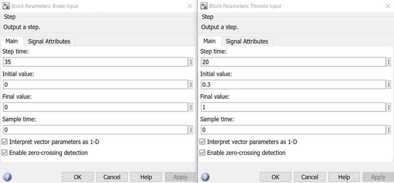
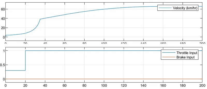
2. Instead of a signal builder for brake and throttle input, In this model step block is used. Throttle input initial value is 0.3 and final value is 1 at 20 sec. Brake input is 0 through out the simulation. Brake Input Throttle Input
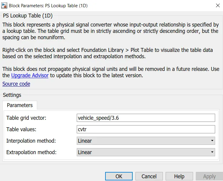
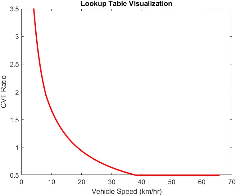
3. And instead of a signal builder for CVT gear ratio, a lookup tabel is used which uses the vehicle speed is used as a feedback signal for the lookup table. The data table is given using matlab workspace. vehicle speed is divided by 3.6 to convert Kph to m/s.
4. Remaning flow process is same as the #1 Model: CVT model.

Output:

1. Engine Torque vs RPM curve:
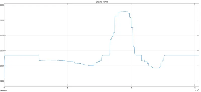
2. Engine RPM vs Time:
3. Lookup Table:
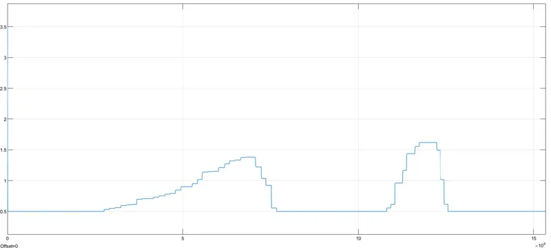
4. CVT Ratio vs Time:
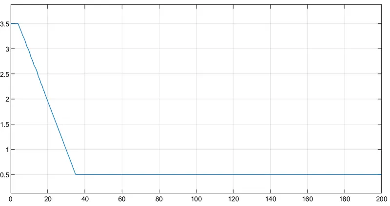
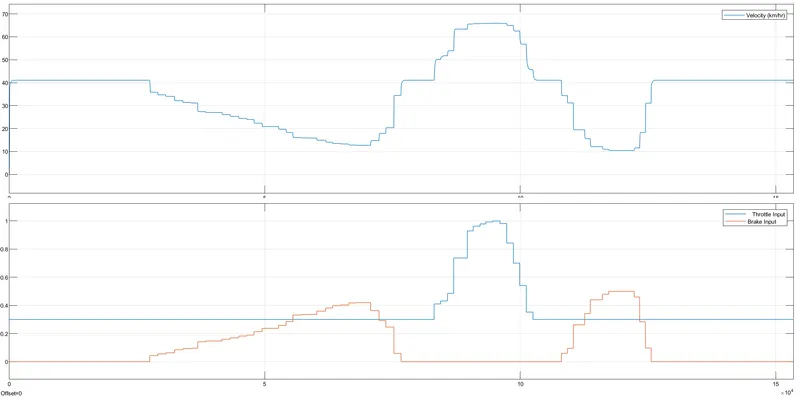
5. Velocity,Throttle, Brake Input vs time:
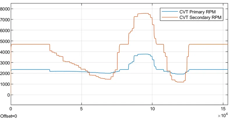
6. CVT gear ratio vs time:

#5 Model CVT model data with dashboard:

Model and Subsystem:

• Model:
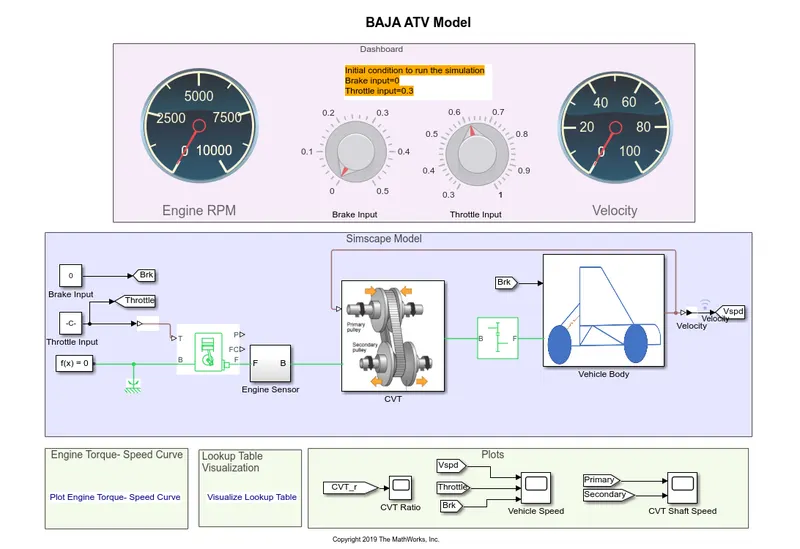
• Subsystems: All the subsystems are same as '#1 Model: CVT model'.

Flowprocess:

1. The Flow process is same as '#4 Model: CVT model'.But the throttle input and brake input are given using user controlled knobs.

Output:

1. Engine Torque vs RPM curve:
2. Engine RPM vs Time:
3. Lookup Table:
4. CVT Ratio vs Time:
5. Velocity,Throttle, Brake Input vs time:
6. CVT gear ratio vs time:

Simulink:

• baja ATV model

References:

• https://www.youtube.com/watch?v=gOFweQcz0XI