Project

Theory

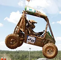
Baja is a small off road vehicle than can withstand harshest elements of rough terrain. It looks similar to dune buggy or beach buggy.

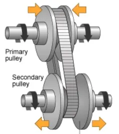
A CVT is an automatic transmission that can change through a continuous range of gear ratios. It may allow the engine to operate at a constant rpm while the vehicles moves at varying speeds. Common type of CVT uses 2 pulleys connected by a belt or chain as shown below.

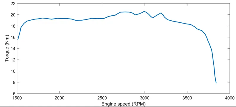
The engine data used in the model is provided as an image which shows the engine speed (RPM) vs torque curve.

Model:

1. BAJA ATV model

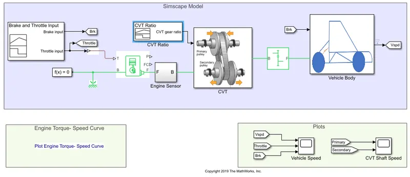
Initially a signal builder is used to provide brake and throttle input to the system. Goto blocks are used to send signals to from blocks that have specified tag. Signal from the signal builder is given below.

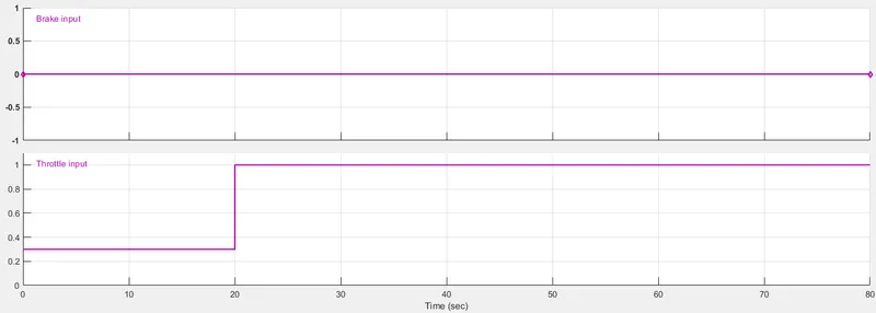
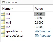
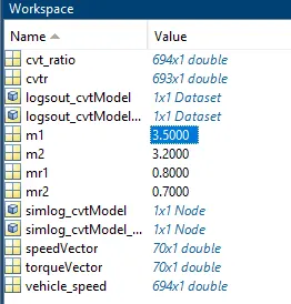
Here, no brake input is given but throttle input is provided. For the first 20s throttle value is 0.3 and for rest of the time its value is 1. Then this output is given to a generic engine block which represents a system level model. The throttle input signal T lies between 0 and 1 and specifies the torque demanded from the engine as a fraction of the maximum possible torque. Connections F and B are mechanical rotational conserving ports associated with the engine crankshaft and engine block respectively. Connections P and FC are physical signal output ports through which engine power and fuel consumption rate are reported. Speed vector and torque vector used in this block are given externally from workspace.

 

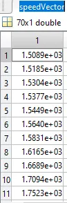
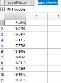
This block is connected to a subsystem named engine sensor. It is represented below.

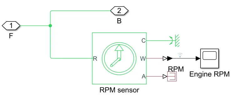
Ideal mechanical rotational motion sensor (rpm sensor) has connections R and C those are mechanical rotational conserving ports and connections W and A are physical signal output ports for velocity and angular displacement respectively. This is connected to a simple gear block followed by a subsystems of CVT and vehicle body respectively.

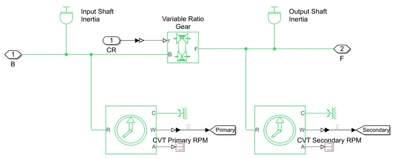
Data's for the input shaft inertia and output shaft inertia (m1 = 3.5  and m2= 3.2) used in CVT subsystem are given through workspace. These inputs are given to a variable ratio gear. It represents a variable ratio gearbox such as implemented by a mechanical belt CVT, electric or hydraulic transmissions. The physical signal input r defines the ratio of input to output angular shaft velocities. Connections B (base) and F (follower) are mechanical rotational conserving ports. Specify the relation between base and follower rotation directions with the output shaft rotation parameter. Two rotational motion sensors are provided to detect the motion of two shafts. Connections R and C are mechanical rotational conserving ports and connections W and A are physical signal output ports for velocity and angular displacement respectively. A signal builder as shown below is used to give gear ratio inputs into CVT subsystem.

As discussed earlier, there is a vehicle body subsystem also. Its model is given below.

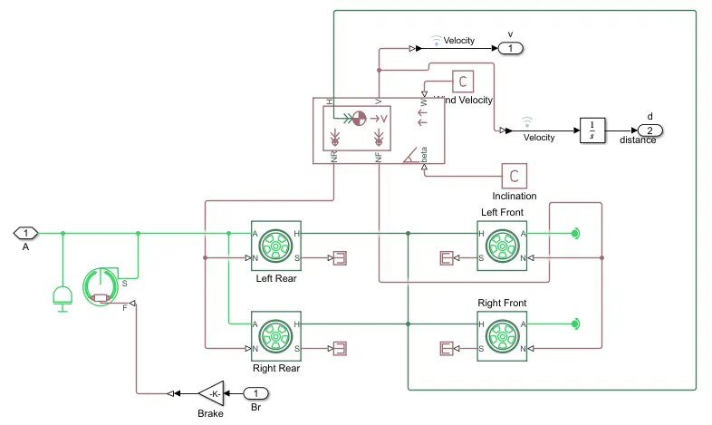
In vehicle body subsystem the main block is vehicle body block. It represents a 2 axle vehicle body in longitudinal motion. Connection H is the mechanical translational conserving port associated with the horizontal motion of the vehicle body. The resulting traction motion developed by tires should be connected to this port. Connections V, NF and NR are physical output ports for vehicle velocity, front and rear normal wheel forces respectively. Wheel forces are considered positive if acting downwards. Connections W and beta are physical signal input ports CG and M are exposed. CG accepts a two element vector representing the x and y distance offsets from vehicle CG to additional load mass CG. M represents the additional mass. If both variable mass and pitch dynamics are included, the physical signal port J accepts the inertia of the additional mass about its own CG. The main parameters given as input are represented below.

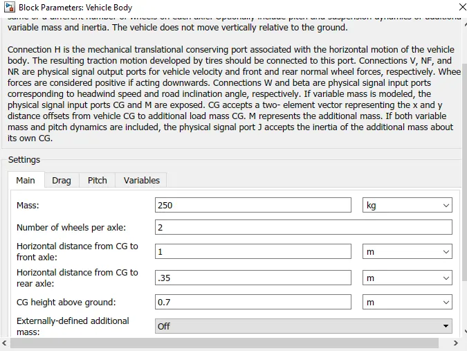
4 tires are connected to a brake drum block. It represents a brake arranged as 2 pivoted rigid shoes symmetrically installed inside or outside a drum and operated by one actuator. The actuator force causes the shoes to exert a friction torque on a shaft connected to the drum. Connection S is a conserving rotational terminal associated with the drum shaft. Connection F is a physical signal port representing the force input to the actuator. Positive force creates friction torque that resists shaft rotation. Its parameters are given below.

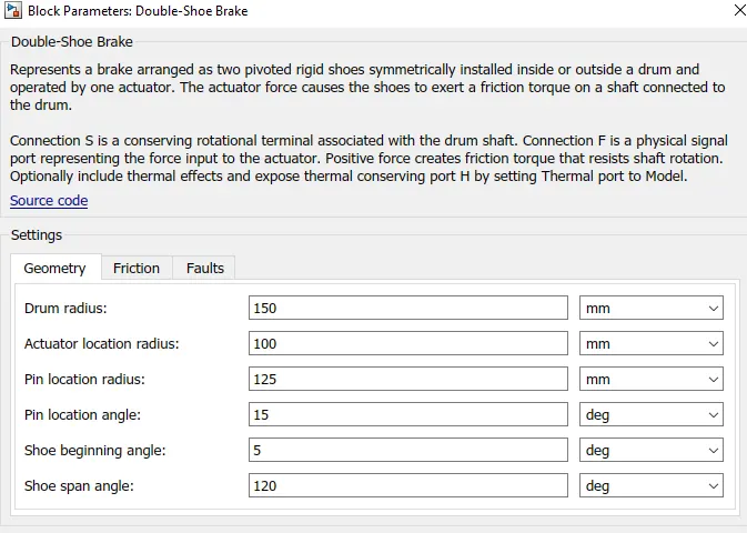
Finally, we will run the simulation and every output is displayed through scope block from which we will analyze the results.

Results:

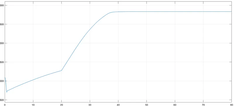
Above graph shows the engine rpm. We gave the throttle input as 0.3 for the first 20 seconds and increased the value to 1 after 20 seconds. So the rpm value was below 2250 during first 20 seconds and increased up to 3800 after 20 seconds. RPM is steady after 40 seconds. Now, the vehicle speed is taken from the scope which is placed externally. It is given below.

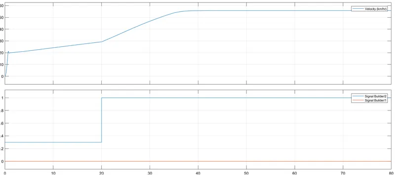
Vehicle speed plot shows that, velocity of the vehicle was similar to the change of rpm. Velocity was below 30 km/hr for first 20 seconds and reached about 58km/hr after 20 seconds. We can also refer that with throttle and brake input in the plot. Shaft speed is also taken from another scope block.

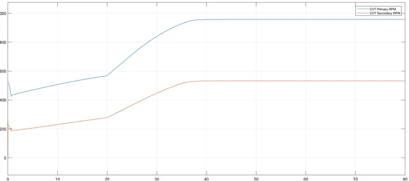
Shaft speed plot is given above. Graph shows the speed of two shafts in CVT. It also behaved like other graphs. Speed was below 600 before 20 seconds and reached about 950 after 40 seconds.

So, from these results we can say that engine rpm, velocity of vehicle and shaft speed is proportional to the throttle input. These values behaves exactly like the value of throttle.

2. BAJA ATV with dashboard. 

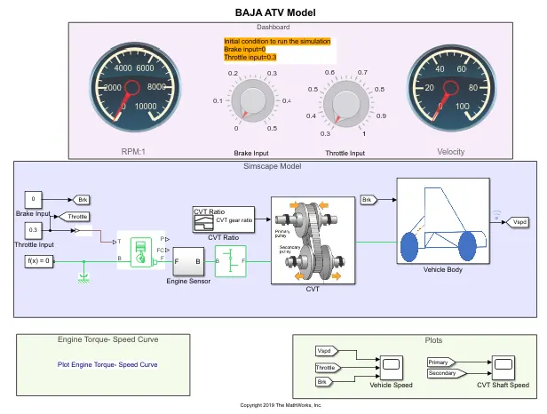
In this model the signal builder which is used to give throttle and brake input is replaced with 2 knobs. By knob block, we can manually change throttle and brake like in a practical situation. Custom gauges and knobs replicate the dashboard. Every other connections are same as the previous model. Initial condition of the dashboard for the simulation is defined as 0 brake input and 0.3 throttle input. Result of the simulation is given below.

Results:

From engine sensor subsystem, we will get the engine rpm plot. It is given below

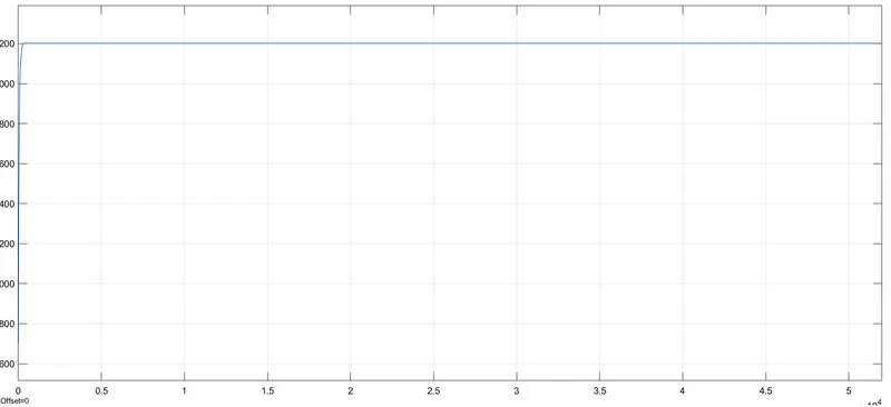
We can observe that the rpm holds a steady value of 3200. Because the throttle input is constant and brake is applied. Now we can predict the vehicle speed same as engine rpm. Vehicle speed plot is given below.

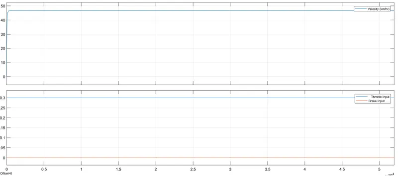
Vehicle speed is also constant because the throttle value is 0.3. Speed was more than 45 km/hr. Shaft speed will also be constant. We can confirm it from the shaft speed plot provided below.

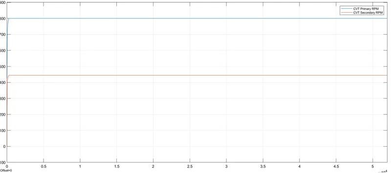
Primary shaft obtained constant value of 800 rpm and secondary shaft speed was 450 rpm.

In this model, we have the facility to vary the input values. So by giving different inputs, we can observe the changes in the plots.

Different input conditions are given to the model and the output is represented below.

Brake input = 0 and throttle input = 1

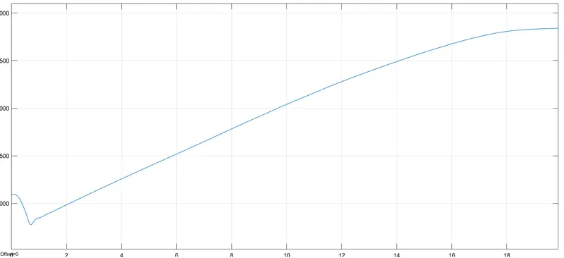
Engine rpm rose up to 3800 when the throttle input was 1. But the rise was not sudden, it was gradual. Now the vehicle speed plot is given below.

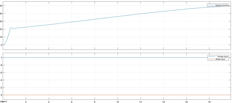
Vehicle speed plot is similar to the plot that we had when there was no dashboard. But when we compare those two here the increase in velocity was quick and reached maximum speed in less time. The shaft speed is given below.

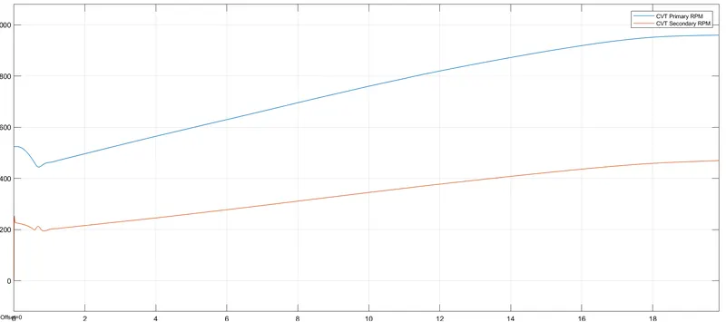
Shaft speed is also same as the first model. Here also the starting was rough but it gained maximum value in less time.

Modeling with the help of lookup table

Lookup table blocks use arrays of data to map input values to output values approximating mathematical functions. Here we use a PS lookup table (1D) block. It computes an approximation to some function with given data vectors. Both input and output will be physical signals. Data vectors provided for this model is having same length and x data vector is monotonic. Then the block generates the simulation. In this model the lookup data visualization is performed and the result is as follows.

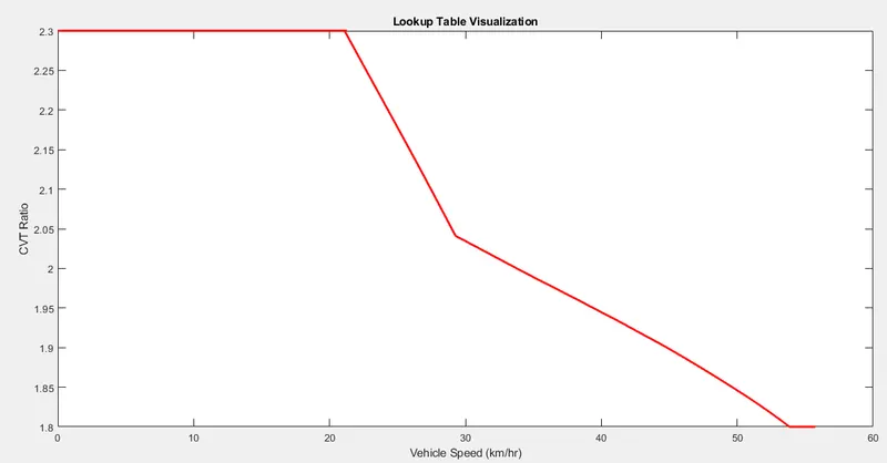
The plot reflects tabulated data specified for the block. Now we can apply the data into the model and simulate the results.

3. BAJA ATV model

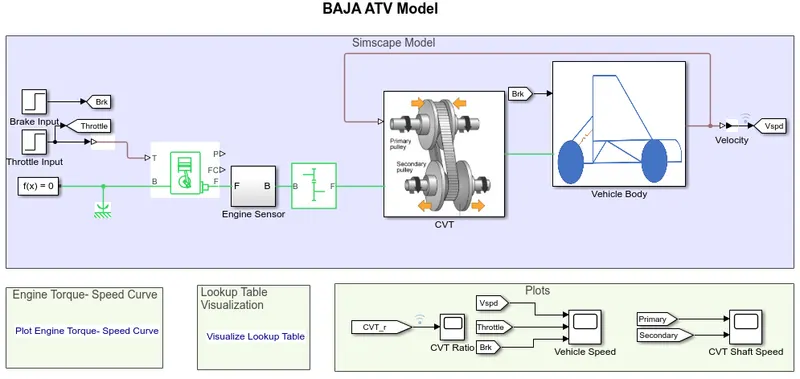
In this model the only difference from the previous model are, the brake and the throttle inputs are given as step block values and the CVT ratio is given through lookup table block. In brake input, the step time is 35 and in throttle input the step time is given as 20. In previous cases, the gear ratios were given to CVT subsystem as signals using signal builder blocks. Here the gear ratios are given externally using lookup tables. For this, a PS lookup table block is inserted in CVT subsystem. Now the simulation performed and the results are plotted below.

Results

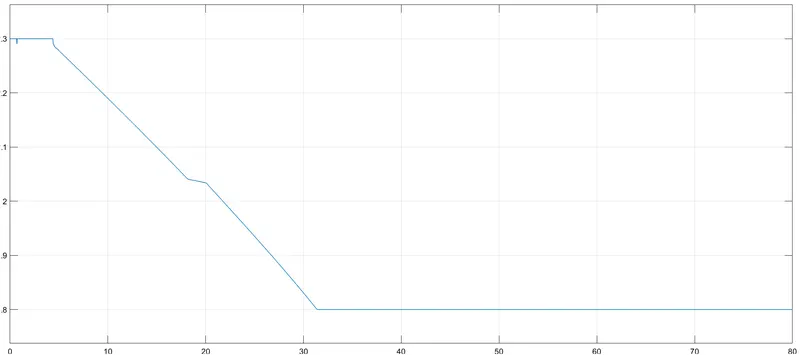
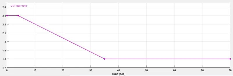
As we can observe from the plot of CVT ratio the value decreased from 2.3 to 1.8 when the speed was above 30. After that it was constant. The decrease is quite straight because we use step input. Now we can look into the vehicle speed for more clarification.

 

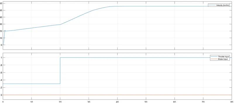
Vehicle speed is suddenly increased after 20s and reached above 55 km/hr when throttle was changed to 1. Shaft speed is represented below.

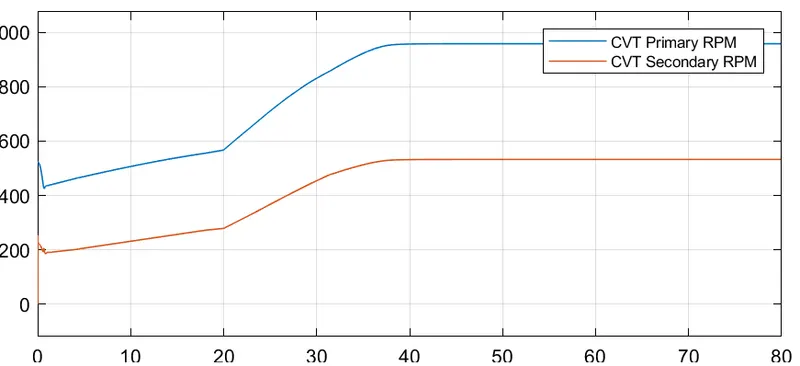
We can observe that shaft speed exactly resembles the plot which have same kind of throttle input. Now we can check out the conditions for the model with dashboard.

4. BAJA ATV with Dashboard

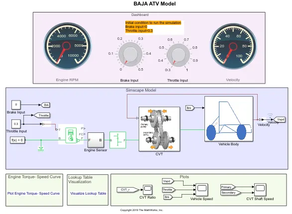
Here the dashboard is made up with 2 knobs and 2 custom gauges. The knobs give brake and throttle input and the gauges represent velocity and rpm. Also like in previous model, CVT system is provided with lookup table block were we give gear ratio inputs. After running the simulation we got the results and they are given below.

Results

We start with the initial condition provided and will change accordingly.

Throttle input = 0.3 and brake input = 0

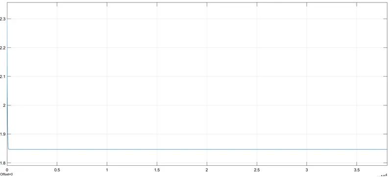
CVT ratio plot is represented above. We can observe that the value has suddenly changed to a constant value of 1.85 when the simulation has been run with 0.3 throttle input.

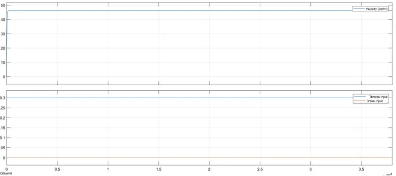
Vehicle speed is constant at about 45km/hr as the throttle input is constant. So that the shaft speed is also constant and it is represented below.

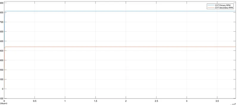
Both shaft speed are constant.

Throttle input = 1 and brake input = 0.5

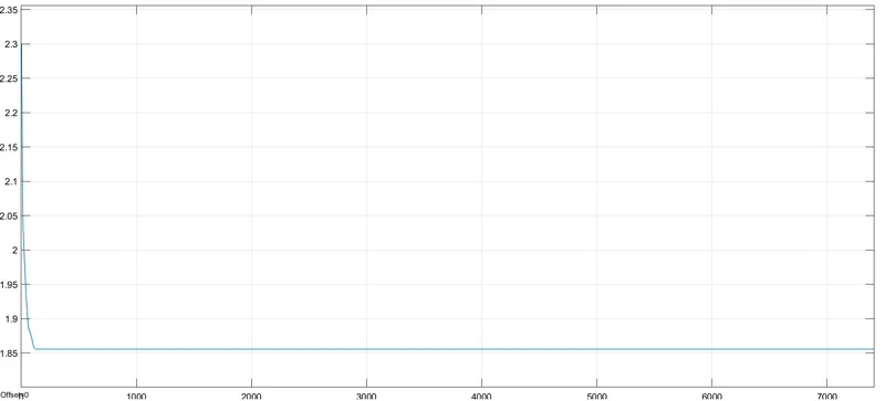
CVT ratio gained the constant value in more time compared to other cases because the brake input is also present. The vehicle speed plot is represented below.

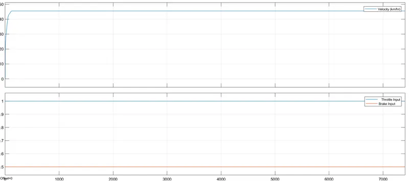
In the starting there are some irregularities in the plot. The brake input tried to resist the velocity but eventually the velocity reached the maximum value. Brake input made the saturation time high.

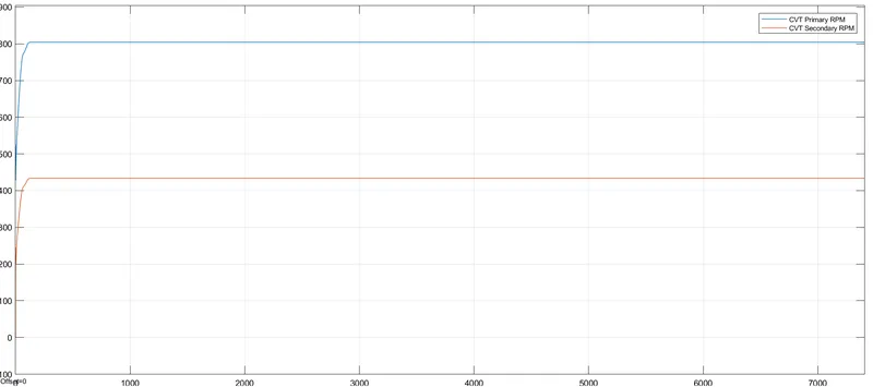
Above graph shows the shaft speed plot and we can observe that the shaft speed is also affected by the brake input.

Conclusion:

Thus we have successfully analyzed 4 different model of BAJA ATV with CVT and recorded the output (vehicle velocity and CVT shaft rom) with respect to variations in input throttle and brake.