Project 1 - Parsing NASA thermodynamic data
AIM:
To write a code in MATLAB to parse NASA thermodynamic data file and then calculate thermodynamic properties of various gas species.
OBJECTIVE:
- Write a function that extracts the 14 coefficients and calculates the enthalpy,entropy and specific heats for all the species in the data file.
- Calculating molecular weight of each species.
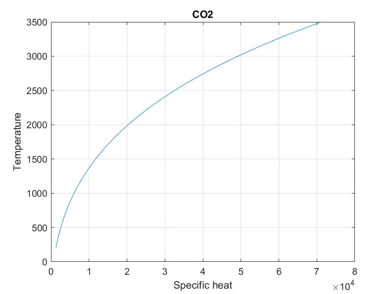
- Plotting the specific heat,enthalpy and entropy for the local temperature range.
- Saving the plots as images with appropriate names and dumping them in seperate folders for each species.
THEORY:
File Parsing :
File parsing is a string or symbol either in natural language, computer language or data structure confirming to the rules of the former grammer.
MATHEMATICAL EQUATION:
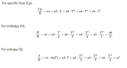
where,
T=local temprature
a1 - a7 = high temperature coefficient
a8 - a14 = low temprature coefficient
R = Universal gas constant = 8.314
14 coefficients are obtained from the thermodynamic data file of which the first 7 are used in low temperature conditions and the latter 7 are used for high temperature conditions. The temperature for each species is mentioned in the data file with a maximum and minimum limit as well as a median limit. For temperatures above the median limit, the high temperature coefficients are used and for temperatures below the median limit, the low temperature coefficients are used.
MATLAB CODE :
MAIN CODE :
clear all
close all
clc

f1=fopen('THERMO.dat','r');

for i=1:5
   fgetl(f1);
end

for i=1:53
tline1=fgetl(f1);
splitline=strsplit(tline1,' ');
species_name=splitline{1};
find_dot=strfind(tline1,'.');
%Line1
local_low_temp=str2double(tline1(find_dot(1)-3:find_dot(1)));
local_high_temp=str2double(tline1(find_dot(2)-4:find_dot(2)));
local_medium_temp=str2double(tline1(find_dot(3)-4:find_dot(3)));

%reading the coefficients
%Line2
tline2=fgetl(f1);
find_e=strfind(tline2,'E');
a1=str2double(tline2(1:find_e(1)+3));
a2=str2double(tline2(find_e(1)+4:find_e(2)+3));
a3=str2double(tline2(find_e(2)+5:find_e(3)+3));
a4=str2double(tline2(find_e(3)+4:find_e(4)+3));
a5=str2double(tline2(find_e(4)+5:find_e(5)+3));

%Line3
tline3=fgetl(f1);
find_e=strfind(tline3,'E');
a6=str2double(tline3(1:find_e(1)+3));
a7=str2double(tline3(find_e(1)+4:find_e(2)+3));
a8=str2double(tline3(find_e(2)+5:find_e(3)+3));
a9=str2double(tline3(find_e(3)+4:find_e(4)+3));
a10=str2double(tline3(find_e(4)+5:find_e(5)+3));

%Line4
tline4=fgetl(f1);
find_e=strfind(tline4,'E');
a11=str2double(tline4(1:find_e(1)+3));
a12=str2double(tline4(find_e(1)+5:find_e(2)+3));
a13=str2double(tline4(find_e(2)+5:find_e(3)+3));
a14=str2double(tline4(find_e(3)+5:find_e(4)+3));

T=local_low_temp:local_high_temp;
%Universal gas constant
R=287;
if T>local_medium_temp
% To calculate Specific heat
Cp=R*(a1+a2*T+a3*T.^2+a4*T.^3+a5*T.^4);
% To calculate Entropy
H=R*(a1+a2*T./2+a3*T.^2./3+a4*T.^3./4+a5*T.^4./5+a6./T).*T;
% To calculate Entropy
S=R*(a1*log(T)+a2*T+a3*T.^2./2+a4*T.^3./3+a5*T.^4./4+a7);
else
% To calculate Specific heat
Cp=R*(a8+a9*T+a10*T.^2+a11*T.^3+a12*T.^4);
% To calculate Entropy
H=R*(a8+a9*T./2+a10*T.^2./3+a11*T.^3./4+a12*T.^4./5+a13./T).*T;
% To calculate Entropy
S=R*(a8*log(T)+a9*T+a10*T.^2./2+a11*T.^3./3+a12*T.^4./4+a14);
end

mw=molecular_weight(species_name);
sprintf('molecular weight of %s=%d',species_name,mw)

mkdir(species_name)
cd(species_name)
figure(1)
plot(Cp,T)
grid on
title(species_name)
xlabel('Specific heat')
ylabel('Temperature')
saveas(1,'CP.png')


figure(2)
plot(H,T)
grid on
title(species_name)
xlabel('Enthalpy')
ylabel('Temperature')
saveas(2,'H.png')


figure(3)
plot(S,T)
grid on
title(species_name)
xlabel('Entropy')
ylabel('Temperature')
saveas(3,'S.png')

cd ..
end
Function code:
function [MW]=molecular_weight(species_name)

elements=['H','C','O','N','R'];
aw=[1,12,16,14,40];

MW=0;
for i=1:length(species_name)
    for j=1:length(elements)
        if strcmp(species_name(i),elements(j))
            MW=MW+aw(j);
            p=j;
        end
    end
     n=str2double(species_name(i));
     if n>1
        MW=MW+aw(p)*(n-1);
     end
end
end
Result :
Molecular weight of all species
ans =

    'molecular weight of O=16'


ans =

    'molecular weight of O2=32'


ans =

    'molecular weight of H=1'


ans =

    'molecular weight of H2=2'


ans =

    'molecular weight of OH=17'


ans =

    'molecular weight of H2O=18'


ans =

    'molecular weight of HO2=33'


ans =

    'molecular weight of H2O2=34'


ans =

    'molecular weight of C=12'


ans =

    'molecular weight of CH=13'


ans =

    'molecular weight of CH2=14'


ans =

    'molecular weight of CH2(S)=14'


ans =

    'molecular weight of CH3=15'


ans =

    'molecular weight of CH4=16'


ans =

    'molecular weight of CO=28'


ans =

    'molecular weight of CO2=44'


ans =

    'molecular weight of HCO=29'


ans =

    'molecular weight of CH2O=30'


ans =

    'molecular weight of CH2OH=31'


ans =

    'molecular weight of CH3O=31'


ans =

    'molecular weight of CH3OH=32'


ans =

    'molecular weight of C2H=25'


ans =

    'molecular weight of C2H2=26'


ans =

    'molecular weight of C2H3=27'


ans =

    'molecular weight of C2H4=28'


ans =

    'molecular weight of C2H5=29'


ans =

    'molecular weight of C2H6=30'


ans =

    'molecular weight of CH2CO=42'


ans =

    'molecular weight of HCCO=41'


ans =

    'molecular weight of HCCOH=42'


ans =

    'molecular weight of H2CN=28'


ans =

    'molecular weight of HCN=27'


ans =

    'molecular weight of HNO=31'


ans =

    'molecular weight of N=14'


ans =

    'molecular weight of NNH=29'


ans =

    'molecular weight of N2O=44'


ans =

    'molecular weight of NH=15'


ans =

    'molecular weight of NH2=16'


ans =

    'molecular weight of NH3=17'


ans =

    'molecular weight of NO=30'


ans =

    'molecular weight of NO2=46'


ans =

    'molecular weight of HCNO=43'


ans =

    'molecular weight of HOCN=43'


ans =

    'molecular weight of HNCO=43'


ans =

    'molecular weight of NCO=42'


ans =

    'molecular weight of CN=26'


ans =

    'molecular weight of HCNN=41'


ans =

    'molecular weight of N2=28'


ans =

    'molecular weight of AR=40'


ans =

    'molecular weight of C3H8=44'


ans =

    'molecular weight of C3H7=43'


ans =

    'molecular weight of CH3CHO=44'


ans =

    'molecular weight of CH2CHO=43'

>>
Screenshot of the window where all the folders are saved

PLOTS :
For O2
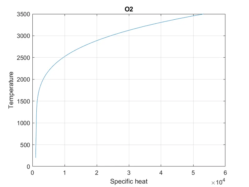
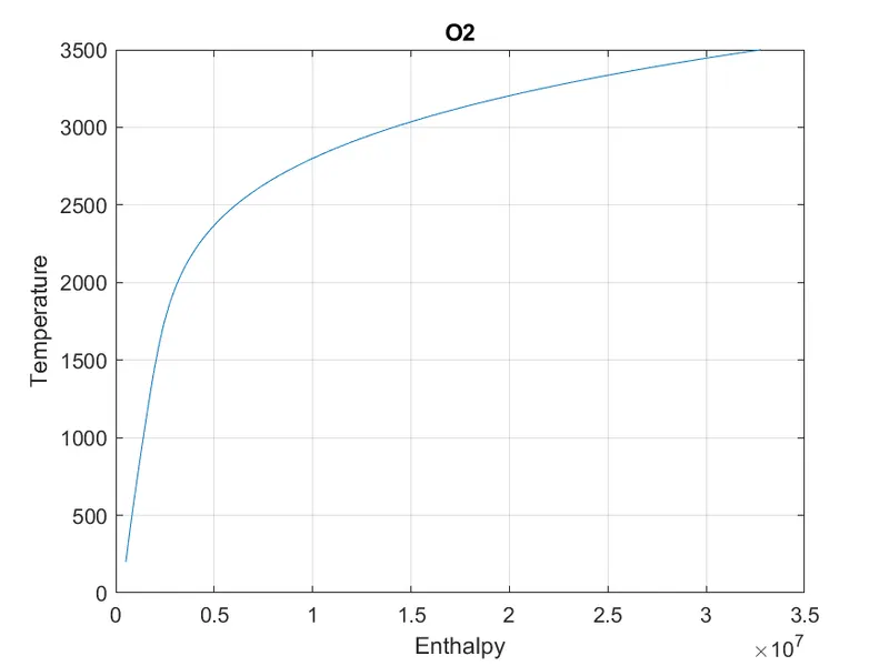
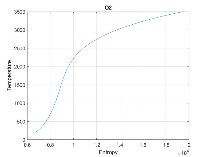
For N2
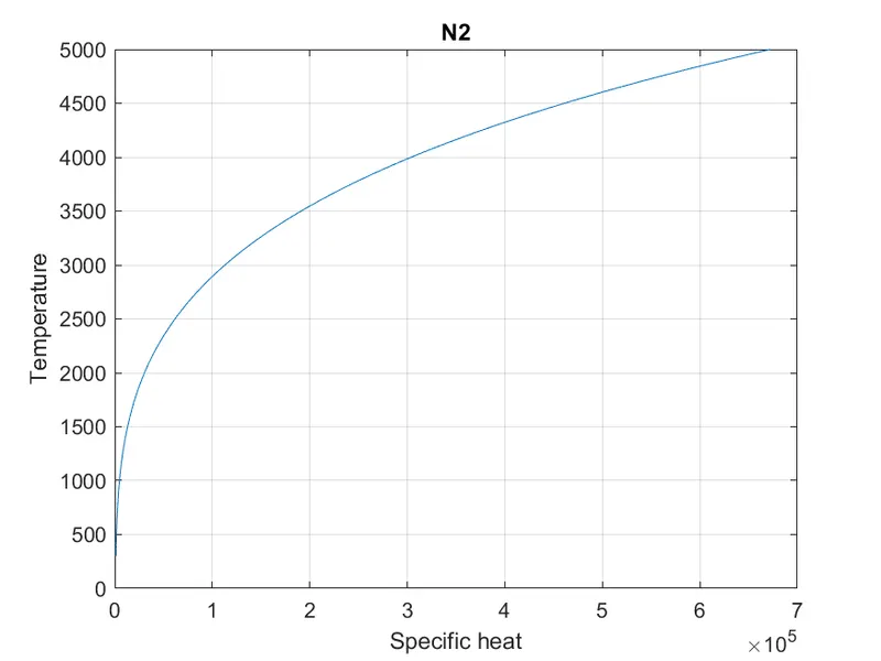
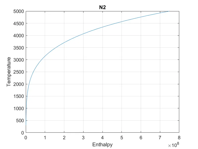
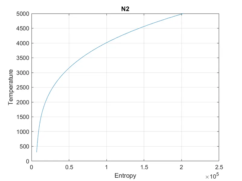
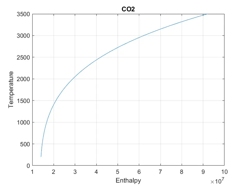
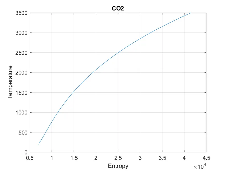
For CO2
CONCLUSION :
- The characteristic curves for all the species are obtained by using MATLAB.
- Cp and S are inversely proportional to temperature they follow a parabolic path and as H is directly proportional to temperature it shows linear plot.