Project 1 - Parsing NASA thermodynamic data

Aim:- To write a function that extracts the coefficients and calculates the enthalpy, entropy, specific heats, and molecular weight for all the species in the data file.

Objectives:-

• To extract the polynomial coefficient of species from the given data file.
• To calculate the enthalpy, entropy, and specific heats for all the species in the data file.
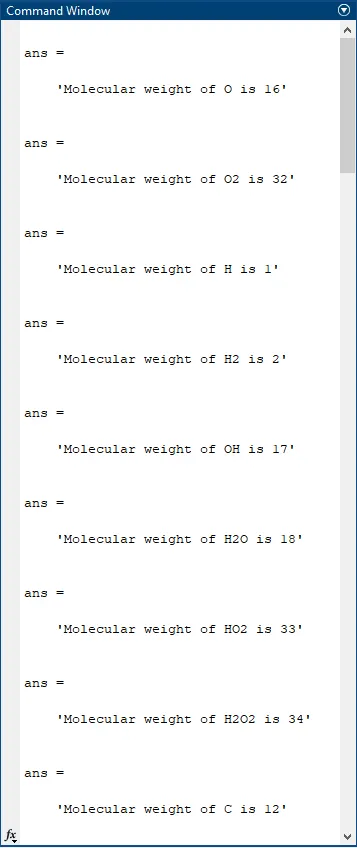
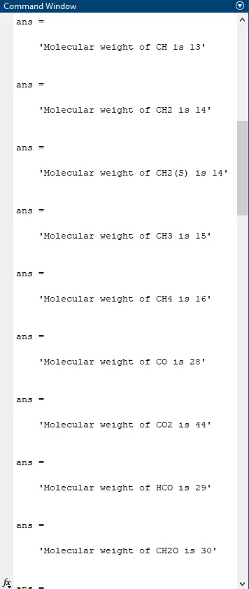
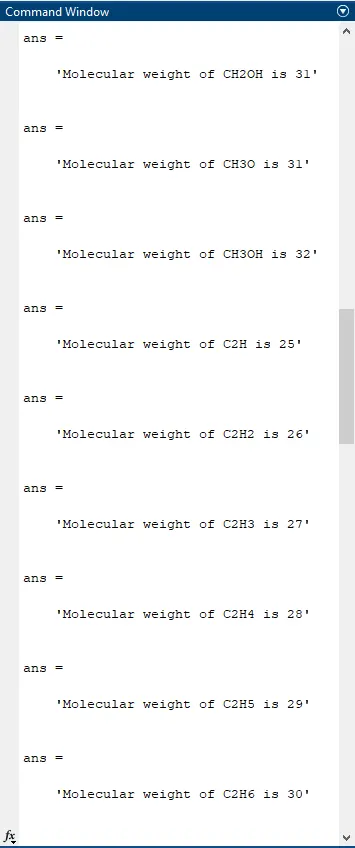
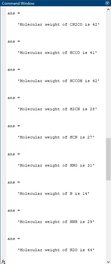
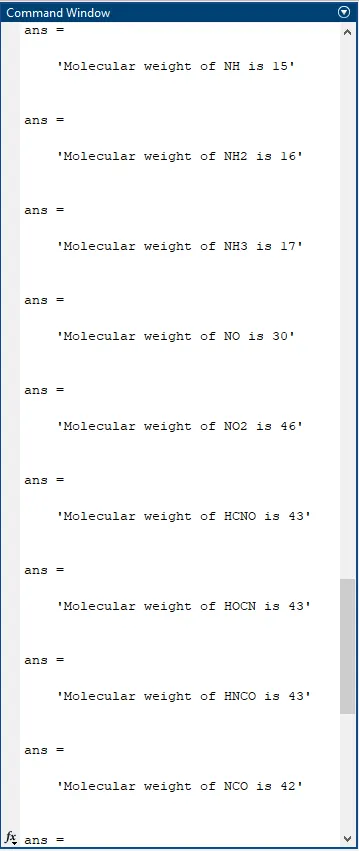
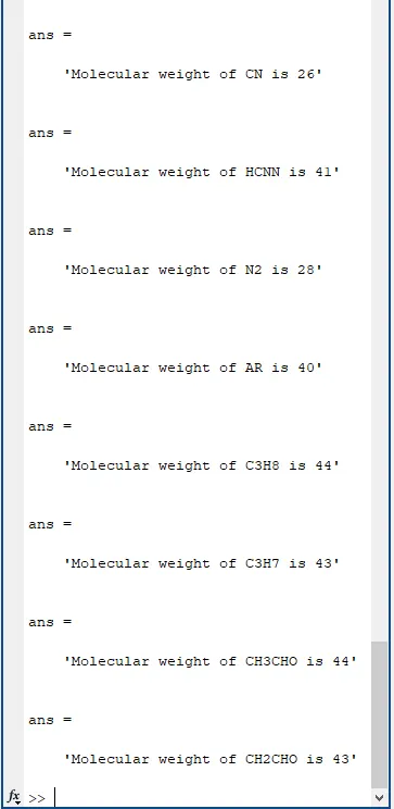
• To calculate the molecular weight of each species and display it in the command window.
• To plot the Cp, Enthalpy, and Entropy for the local temperature range specified for each species.
• To plot a graph diagram for o2, N2, and Co2 species.

Theory:-

What is parsing:-

Parsing, syntax analysis, or syntactic analysis is the process of analyzing a string of symbols, either in natural languages, computer languages, or data structure, conforming to the rules of formal grammar.

Specific Heat (Cp):-

The specific heat is the amount of heat per unit mass required to raise the temperature by one degree Celsius. The relationship between heat and temperature change is usually expressed in the form shown below where c is the specific heat. The relationship does not apply if a phase change is encountered, because the heat added or removed during a phase change does not change the temperature.

Enthalpy(H):-

enthalpy, the sum of the internal energy and the product of the pressure and volume of a thermodynamic system. Enthalpy is an energy-like property or state function—it has the dimensions of energy and its value is determined entirely by the temperature, pressure, and composition of the system and not by its history.

Entropy(S):-

entropy, the measure of a system’s thermal energy per unit temperature that is unavailable for doing useful work. Because work is obtained from ordered molecular motion, the amount of entropy is also a measure of the molecular disorder, or randomness, of a system.

Molecular Weight:-

molecular weight, also called molecular mass, is the mass of a molecule of a substance, based on 12 as the atomic weight of carbon-12. It is calculated in practice by summing the atomic weight of the atoms making up the substance’s molecular formula. The molecular weight of a hydrogen molecule (chemical formula H₂) is 2 (after rounding off); for many complex organic molecules (e.g., proteins, polymers) it may be in the millions.

Governing Equation:-

In the above data, it is specified that the first seven coefficients are high-temperature coefficients and the second seven coefficients are low-temperature coefficients.

Here R is the universal gas constant, T is the temperature

above equation is for the first seven coefficients of high-temperature coefficients.

For the second seven coefficients of low-temperature coefficients. Just change the values of a coefficients to

MATLAB Program:-

To get the desired output as mentioned in the question we need to create two codes first is the function code and the main code.

Function Code:-

% Function To Calculate Molecular Weight

function MW=molecular_weight(species)
elements=['O','H','C','R','N'];

% providing atomic weight of 
% 0XYGEN(16), H=HYDROGEN(1),C=CARBON(12),R=ARGON(40),N=NITROGEN(14)

atomic_weight=[16,1,12,40,14];

  MW=0;
  
 for i=1: length(species)
     
   for j=1:length(elements)
       
if (strcmp(species(i),elements(j))) 
MW = MW + atomic_weight(j);
p=j;

end
   end
   
N=str2double(species(i));

if N>1
    MW=MW+atomic_weight(p)*(N-1);
end 

end

• To calculate the molecular weight of given species used this function command, we used this function command in a separate script file.
• here we use the function command to provide the input values and output arrays to our main program with the help of this we can easily get the values.
• The formula we used in the function command is MW=molecular_weight(species)
• In this command we have given basic elements which are elements=['O','H','C','R','N'] with there atomic weights. The atomic weight of given elements are for 0XYGEN(16), H=HYDROGEN(1),C=CARBON(12),R=ARGON(40),N=NITROGEN(14).
• the molecular weight of species depends on the common atomic weight of elements. After providing the atomic weight we applied for a loop.
• In for loop i=1: length(species) and another for loop are given which means this is nested for loop system where we have j=1:length(elements).
• With the help of the If else system using string compare command, we compared species with respect to i and elements with respect to j.
• And we provided a condition where MW = MW + atomic_weight(j) and the other condition is p=j where p is the position of the element.
• with this, we ended the if-else system as well as for loop for j with end command.
• Again with the help of string2double command, we have the condition of N=str2double(species(i)) where N is the position of numeric value.
• again with the help of the if-else system if the value is less than 1 then MW=MW+atomic_weight(p)*(N-1) this command will be valid.
• with this, we ended the if-else system as well as for loop for i with end command.
• And now we will be able to call this function in our main program code.

Main Program:-

clear all
close all
clc

% Parsing thermal data
f1=fopen('THERMO.dat','r');

for i=1:5
fgetl(f1);
end

for j=1:53
% to split the line    
tline1=fgetl(f1);
splitline=strsplit(tline1,' ');
species = splitline{1};

% finding local temperature

findingdot=strfind(tline1,'.');

low_local_temp=str2double(tline1(findingdot(1)-3:findingdot(1)));
high_local_temp=str2double(tline1(findingdot(2)-4:findingdot(2)));
mid_local_temp=str2double(tline1(findingdot(3)-4:findingdot(3)));

% finding coordinates of line 2

tline2=fgetl(f1);
findingE=strfind(tline2,'E');

a1=str2double(tline2(1:findingE(1)+3));
a2=str2double(tline2(findingE(1)+4:findingE(2)+3));
a3=str2double(tline2(findingE(2)+4:findingE(3)+3));
a4=str2double(tline2(findingE(3)+4:findingE(4)+3));
a5=str2double(tline2(findingE(4)+4:findingE(5)+3));

% finding coordinates of line 3

tline3=fgetl(f1);
findinge=strfind(tline3,'E');

a6=str2double(tline3(1:findinge(1)+3));
a7=str2double(tline3(findinge(1)+4:findinge(2)+3));
a8=str2double(tline3(findinge(2)+4:findinge(3)+3));
a9=str2double(tline3(findinge(3)+4:findinge(4)+3));
a10=str2double(tline3(findinge(4)+4:findinge(5)+3));

% finding coordinates of line 4

tline4=fgetl(f1);
finding_e=strfind(tline4,'E');

a11=str2double(tline4(1:finding_e(1)+3));
a12=str2double(tline4(finding_e(1)+4:finding_e(2)+3));
a13=str2double(tline4(finding_e(2)+4:finding_e(3)+3));
a14=str2double(tline4(finding_e(3)+4:finding_e(4)+3));

% universal gas constant
R = 8.314;

% finding cp enthalpy and entropy 

T=low_local_temp:high_local_temp;

if T>mid_local_temp

cp=R*(a1+(a2*T)+(a3*(T.^2))+(a4*(T.^3))+(a5*(T.^4)));
H=R*(a1+((a2*T)./2)+(a3*(T.^2)./3)+(a4*(T.^3)./4)+(a5*(T.^4)./5)+a6./T);
S=R*((a1*log(T))+(a2*T)+(a3*(T.^2)./2)+(a4*(T.^3)./3)+(a5*(T.^4)./4)+a7);
    
else    
    
cp= R*(a8+(a9*T)+(a10*(T.^2))+(a11*(T.^3))+(a12*(T.^4)));
H=R*(a8+((a9*T)./2)+(a10*(T.^2)./3)+(a11*(T.^3)./4)+(a12*(T.^4)./5)+a13./T);
S=R*((a8*log(T))+(a9*T)+(a10*(T.^2)./2)+(a11*(T.^3)./3)+(a12*(T.^4)./4)+a14);
end 

% To find the molecular weight of species
M=molecular_weight(species);
sprintf('Molecular weight of %s is %d',species,M)

% to make indivisual folders of species
t=sprintf('%s',species);
mkdir(t)
cd(t)

% plotting temperature vs cp diagram
figure(1)
plot(T,cp)
grid on
xlabel('temperature(T)')
ylabel('Specific heat(cp)')
title(sprintf('species name %s',species))
saveas(1,'temperature vs specific heat.jpg')


% plotting temperature vs enthalpy diagram
figure(2)
plot(T,H)
grid on
xlabel('temperature(T)')
ylabel('enthalpy(H)')
title(sprintf('species name %s',species))
saveas(2,'temperature vs enthalpy.jpg')


% plotting temperature vs entropy diagram
figure(3)
plot(T,S)
grid on
xlabel('temperature(T)')  
ylabel('entropy(S)')
title(sprintf('species name %s',species))
saveas(3,'temperature vs entropy.jpg')

cd ..

end

• First, we use the clear all, close all, and clc commands to clear all the unwanted data in the workspace and the command window and close background plots.
• For parsing the given NASA data we used the Fopen command as f1=fopen('THERMO.dat','r') where f1 is going to be assigned data and THERMO.dat is the file name with its file type and r is used to read the file.
• Then we used for loop to skip the first five lines in the given data file and with this for loop is ended using the end command.
• Again another for loop is used where j=53 where 53 is the total number of species.
• fgetl command is used to get the values in the sixth line of given data as we can use this command to skip the line as well.
• then string split command is used as splitline=strsplit(tline1,' '); where thline 1 is the line from which we are extracting the required data and ' ' represents that we are splitting the data according to this.
• With this we got our first species as species = splitline{1} here curly brackets are used to extract species with proper type.
• Then to extract the local temperature values as for low_local_temp=str2double(tline1(findingdot(1)-3:findingdot(1)));
  high_local_temp=str2double(tline1(findingdot(2)-4:findingdot(2)));
  mid_local_temp=str2double(tline1(findingdot(3)-4:findingdot(3)));
• with this we get the local temperature values for low local temperature, mid local temperature and high local temperature.
• Then to find the coordinates of the species of second row first we find there common reference as variable E and using string find command as findingE=strfind(tline2,'E') with this we get our reference point location.
• then using str2double command we extract all the five values from second row as a1=str2double(tline2(1:findingE(1)+3));
  a2=str2double(tline2(findingE(1)+4:findingE(2)+3));
  a3=str2double(tline2(findingE(2)+4:findingE(3)+3));
  a4=str2double(tline2(findingE(3)+4:findingE(4)+3));
  a5=str2double(tline2(findingE(4)+4:findingE(5)+3));
• Reapaing same logic to extract coordinates from third and fourth line we get our coordinates for third row we used a6=str2double(tline3(1:findinge(1)+3));
  a7=str2double(tline3(findinge(1)+4:findinge(2)+3));
  a8=str2double(tline3(findinge(2)+4:findinge(3)+3));
  a9=str2double(tline3(findinge(3)+4:findinge(4)+3));
  a10=str2double(tline3(findinge(4)+4:findinge(5)+3));
• Also for fourth row a11=str2double(tline4(1:finding_e(1)+3));
  a12=str2double(tline4(finding_e(1)+4:finding_e(2)+3));
  a13=str2double(tline4(finding_e(2)+4:finding_e(3)+3));
  a14=str2double(tline4(finding_e(3)+4:finding_e(4)+3));
• Using above commands we extract our coordinate as well as local temperature of species O.
• Then the universal gas constant value is provided as R = 8.314 where R is a constant value.
• To find the values of specific heat enthalpy and entropy we have to find the total temperature of species we can find this using T=low_local_temp:high_local_temp.
• Then if else system is used where if T>mid_local_temp then to find the values of specific heat enthalpy and entropy we have to use formulas for higher local temperature as cp=R*(a1+(a2*T)+(a3*(T.^2))+(a4*(T.^3))+(a5*(T.^4)));
  H=R*(a1+((a2*T)./2)+(a3*(T.^2)./3)+(a4*(T.^3)./4)+(a5*(T.^4)./5)+a6./T);
  S=R*((a1*log(T))+(a2*T)+(a3*(T.^2)./2)+(a4*(T.^3)./3)+(a5*(T.^4)./4)+a7);
• or else when Tthen to find the values of specific heat enthalpy and entropy we have to use formulas for higher local temperature as cp= R*(a8+(a9*T)+(a10*(T.^2))+(a11*(T.^3))+(a12*(T.^4)));
  H=R*(a8+((a9*T)./2)+(a10*(T.^2)./3)+(a11*(T.^3)./4)+(a12*(T.^4)./5)+a13./T);
  S=R*((a8*log(T))+(a9*T)+(a10*(T.^2)./2)+(a11*(T.^3)./3)+(a12*(T.^4)./4)+a14)
• By using this formulas we are able to find the values of specific heat enthalpy and entropy with respect to there temperature.
• To find the molecular weight of species we have to call our function command from function code as we mentioned earlier than to print the answer values of every species we used sprintf command as sprintf('Molecular weight of %s is %d',species,M) with this commands we are able to get the molecular weight of our species.
• Then to make individual folders of species to store their specific heat enthalpy and entropy curves we used sprintf command as t=sprintf('%s',species) where t is assigned variable to represent and %s represents string operator.
• The mkdir(t) the make directory command is used to make a path to create new folders with respect to the species.
• Then cd(t) is used to close the directory which is created by mkdir command.
• To plot the temperature vs cp diagram we used plot command as plot(T,cp) then to plot temperature vs enthalpy diagram we used plot(T,H), and to plot temperature vs entropy diagram we used plot(T,S)
• Then grid on command is used to get grid views of the graph.
• xlabel and ylabel commands are used to give names to the axis of graphs.
• then title command is used to name the graph with respect to their species name as the title(sprintf('species name %s',species)).
• saveas command is used to save the plotted graph in their manner.
• then cd.. is used to close that directory which is opened.
• And we ended our for loop here with end command.
• After writing all the code successfully we have to run the program. With this, we get our output successfully.

Output/Result:-

plots of specific heat enthalpy and entropy for o2:-

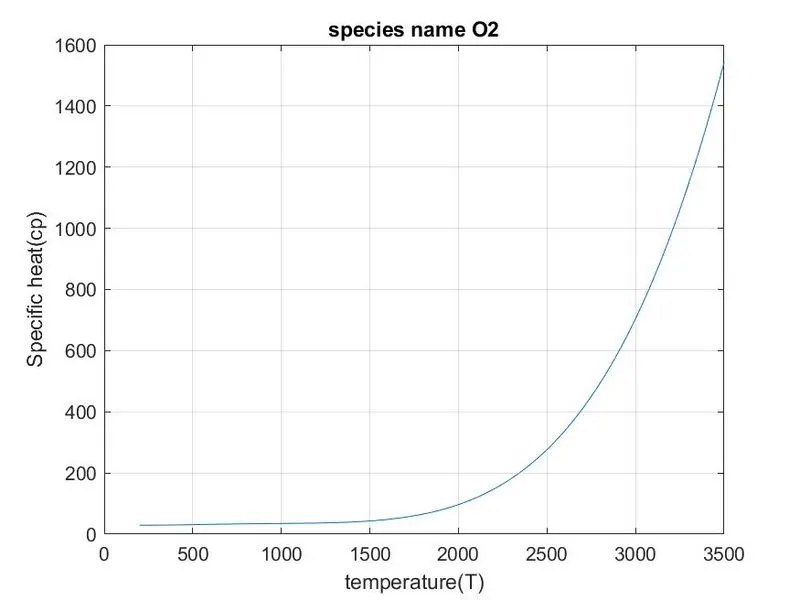
The above diagram is the temperature vs specific heat of O2 species.

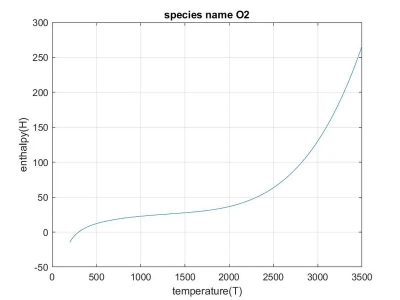
The above diagram is the temperature vs enthalpy of O2 species.

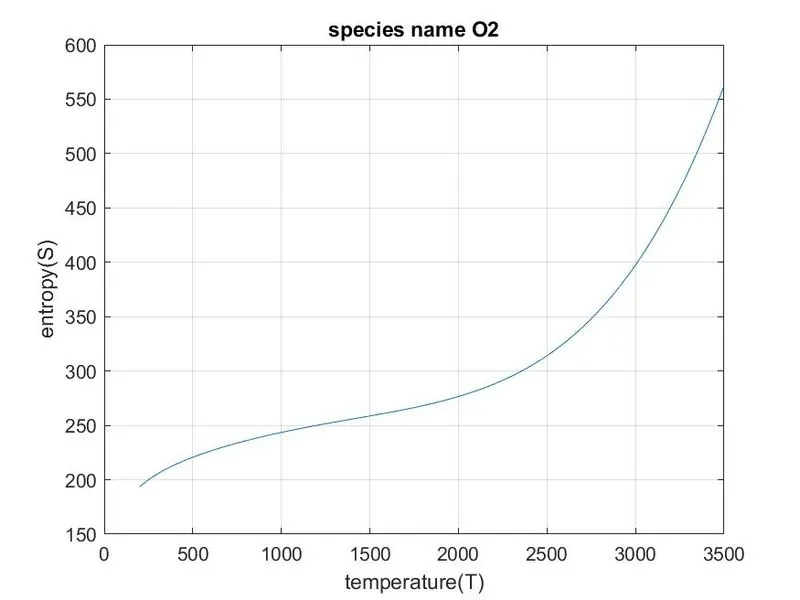
The above diagram is the temperature vs entropy of O2 species.

plots of specific heat enthalpy and entropy for N2:-

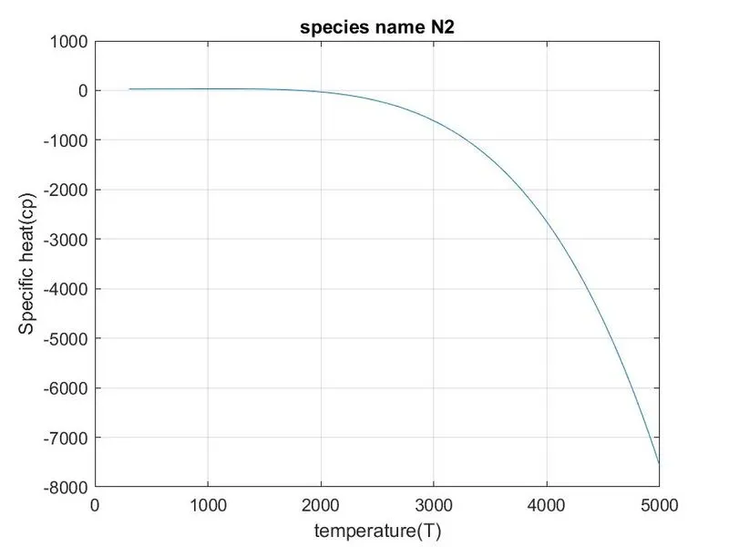
The above diagram is the temperature vs specific heat of N2 species.

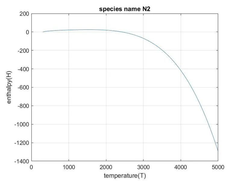
The above diagram is the temperature vs enthalpy of N2 species.

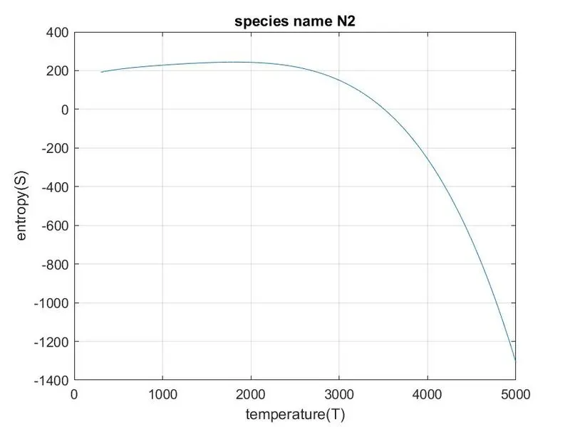
The above diagram is the temperature vs entropy of N2 species.

plots of specific heat enthalpy and entropy for CO2:-

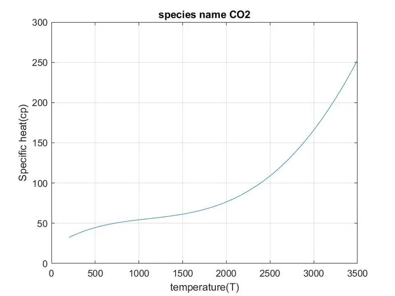
The above diagram is the temperature vs specific heat of CO2 species.

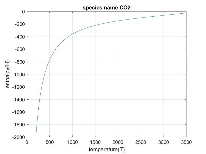
The above diagram is the temperature vs enthalpy of CO2 species.

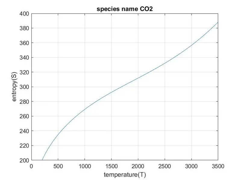
The above diagram is the temperature vs entropy of CO2 species.

Molecular Weight Of Species:-

Screenshot Where all Folders are saved:-

Conclusion:-

With the help of MATLAB, we extract all the 14 coefficients of 53 species as given in the data file also calculated their individual specific heat enthalpy and entropy and along with their curves with respect to temperature Successfully.