Project 1 - Parsing NASA thermodynamic data

PARSING NASA THERMODYNAMICS DATA

• Write a function that extracts the 14 coefficients and calculates the enthalpy, entropy, and specific heats for all the species in the data file. You will be reading this file NASA thermodynamic data (Tip: use fopen and fgetl). The formulae are shown below.

  Here R is the universal gas constant, T is the temperature

  The FIRST 7 coefficients are HIGH-temperature coefficients and the SECOND 7 coefficients are LOW-temperature coefficients.

• % Writing the code for extracting the 14 coefficients value and to find cp,
  % H, S
  clear all
  close all
  clc
  
  %To open Data file
  f = fopen('THERMO.dat','r')
  % To read first five lines
  for i = 1:5
      fgetl(f);
  end
  
  %extracting all the 53 species
  for j = 1:53
  
   % To get element_name    
   a = fgetl(f);
   element_name = strtok(a);
   b = strsplit(a,' ');
  
   % To extract the locallow,mid,high temperature
  local_low = str2num(b{end-3});
  local_high = str2num(b{end-2});
  local_mid = str2num(b{end-1});
     
  
  % To extract all the 14 coefficient values.
  coeff_line1 = fgetl(f);
  pos_e = strfind(coeff_line1,'E');
  
  a1 = str2num(coeff_line1(1:pos_e(1)+3));
  
  a2 = str2num(coeff_line1(pos_e(1)+4:pos_e(2)+3));
  a3 = str2num(coeff_line1(pos_e(2)+4:pos_e(3)+3));
  a4 = str2num(coeff_line1(pos_e(3)+4:pos_e(4)+3));
  a5 = str2num(coeff_line1(pos_e(4)+4:pos_e(5)+3));
  
  coeff_line2 = fgetl(f);
  pos_e1 = strfind(coeff_line2,'E');
  
  a6 = str2num(coeff_line1(1:pos_e(1)+3));
  a7 = str2num(coeff_line1(pos_e(1)+4:pos_e(2)+3));
  b1 = str2num(coeff_line1(pos_e(2)+4:pos_e(3)+3));
  b2 = str2num(coeff_line1(pos_e(3)+4:pos_e(4)+3));
  b3 = str2num(coeff_line1(pos_e(4)+4:pos_e(5)+3));
  
  coeff_line3 = fgetl(f);
  pos_e1 = strfind(coeff_line3,'E');
  
  b4 = str2num(coeff_line1(1:pos_e(1)+3));
  b5 = str2num(coeff_line1(pos_e(1)+4:pos_e(2)+3));
  b6 = str2num(coeff_line1(pos_e(2)+4:pos_e(3)+3));
  b7 = str2num(coeff_line1(pos_e(3)+4:pos_e(4)+3));
  
  %to create new directory and creating seprate folder
  cd('C:\Users\admin\Documents\MATLAB')
  dir_name = element_name;
  mkdir(dir_name);
  cd(element_name)
  
  % To find the molecular weight of 53 species
  molecule_name = molecular_weight(element_name)
  
  % assigning the T value 
  T = linspace(local_low,local_high,100);
  
  % to get values of cp,H,S
     [cp,H,S]= therm_prop(a1,a2,a3,a4,a5,a6,a7,b1,b2,b3,b4,b5,b6,b7,local_mid,T);
  
  %plotting
  
     figure(1)
     plot(T,cp)
     xlabel('Temperature')
     ylabel('Specific Heat')
     saveas(figure(1),'Temperature vs specific heat.jpg')
  
     figure(2)
     plot(T,H,'color','r')
     xlabel('Temperature')
     ylabel('Entalpy')
     saveas(figure(2),'Temperature vs Enthalpy.jpg')
  
     figure(3)
     plot(T,S,'color','g')
     xlabel('Temperature')
     ylabel('Entropy')
     saveas(figure(3),'Temperature vs Entropy.jpg')
     cd ..
      
  end

• Here, I'm using two inside function "therm_prop" and "molecular_weight" in the above code and it can be given as:

1. therm_prop:

%FUNCTION FOR SPECIFIC HEAT,ENTHALPY,ENTROPY

function [cp,H,S] = therm_prop(a1,a2,a3,a4,a5,a6,a7,b1,b2,b3,b4,b5,b6,b7,local_mid,T)
R = 8.314;

if(T<=local_mid)
   
    cp = R.*(b1+b2*T+b3*T.^2+b4*T.^3+b5*T.^4);
    H = R.*T.*(b1+b2*(T/2)+b3*((T.^2)./3)+b4*((T.^3)./4)+b5*((T.^4)./5)+b6./T);
    S = R.*(b1*log(T)+b2*T+b3*((T.^2)./2)+b4*((T.^3)./3)+b5*((T.^4)./4)+b7);
    
else
    cp = R.*(a1+a2*T+a3*T.^2+a4*T.^3+a5*T.^4);
    H = R.*T.*(a1+a2*(T/2)+a3*((T.^2)./3)+a4*((T.^3)./4)+a5*((T.^4)./5)+a6./T);
    S = R.*(a1*log(T)+a2*T+a3*((T.^2)./2)+a4*((T.^3)./3)+a5*((T.^4)./4)+a7);

end

end

2. molecular_weight:

function MW =molecular_weight(element_name)
atoms = ['H','C','N','O','A'];
     fprintf('Molecular Weight of ');
    fprintf(element_name);
    fprintf(' : ');
    atomic_weight = [1 12 14 16 39];
    MW = 0;
    for i = 1:length(element_name)
        for j = 1:length(atoms)
            if strcmp(element_name(i),atoms(j))
                MW = MW +atomic_weight(j);
                position = j;
            end
        end
        n = str2num(element_name(i));
        if n>1
            MW = MW + atomic_weight(position)*(n-1);
        end
    end
    fprintf('%d',MW);
    disp(' ');
    end

• RESULTS:

1. O2

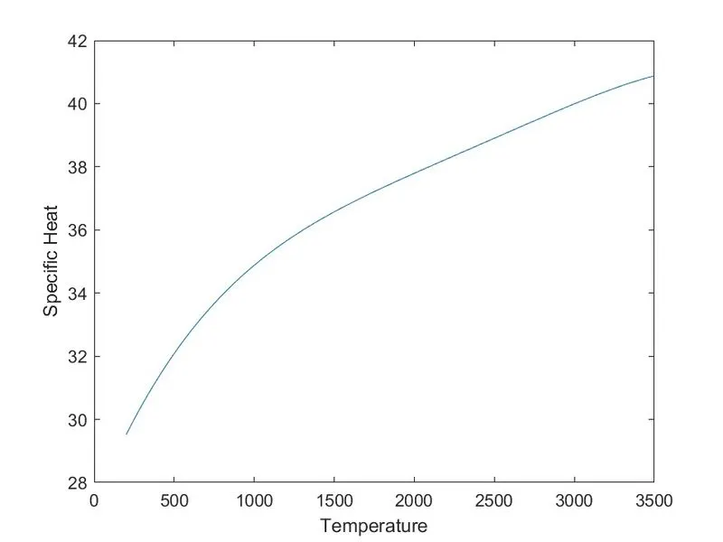
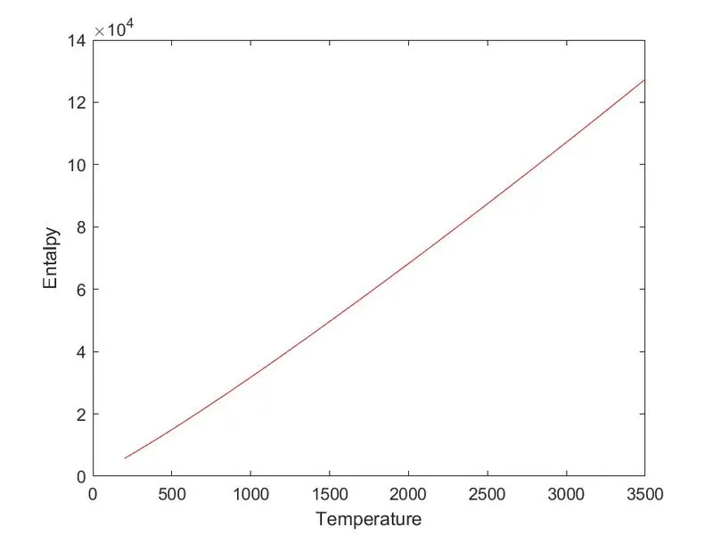
N2

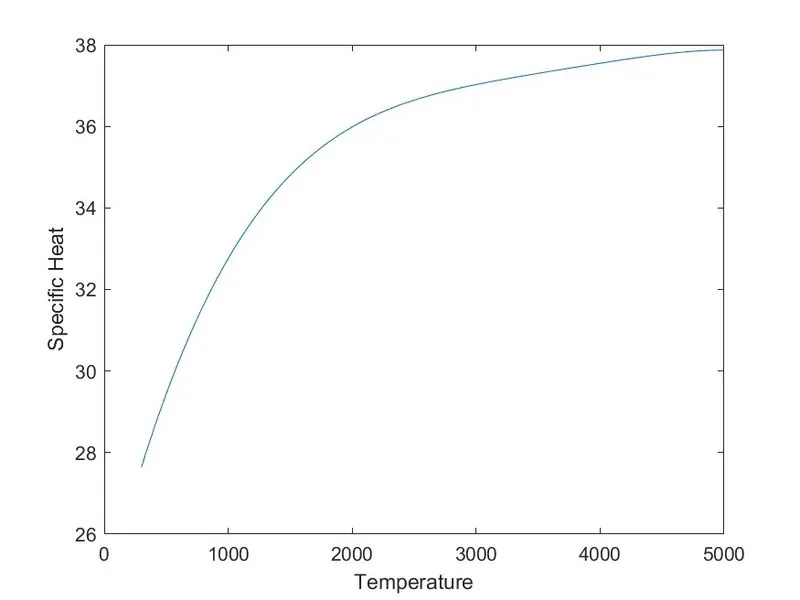
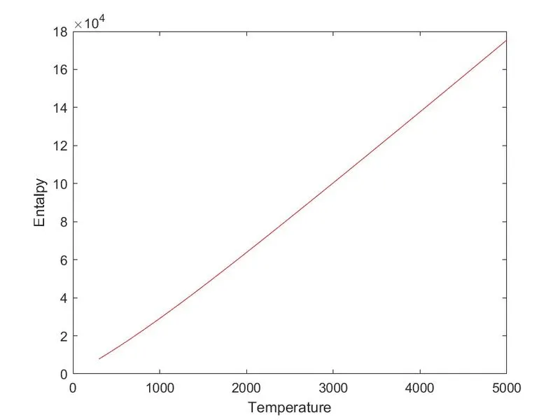
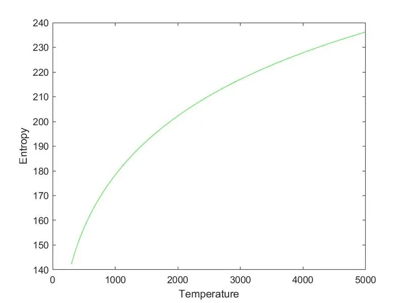
3.CO2

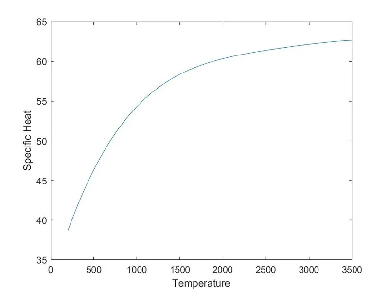
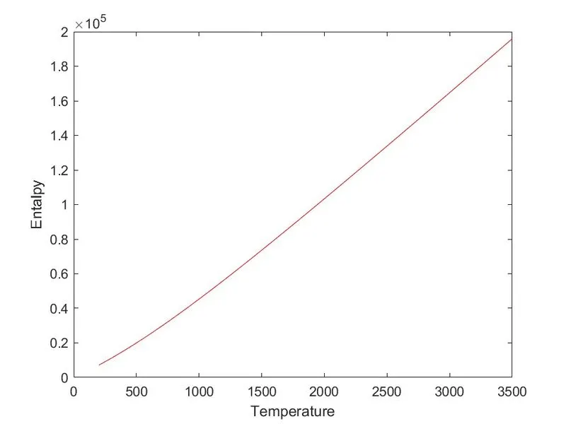
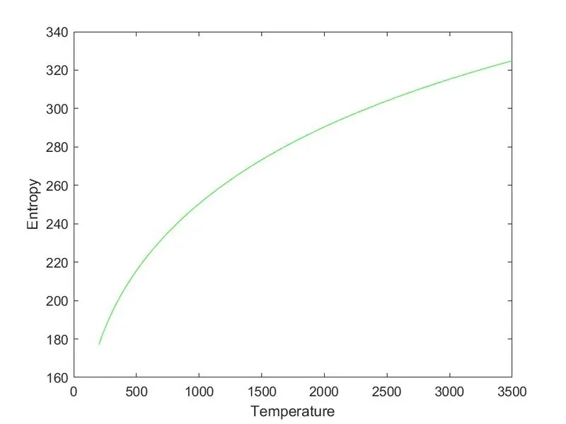
• molecular weight of species:

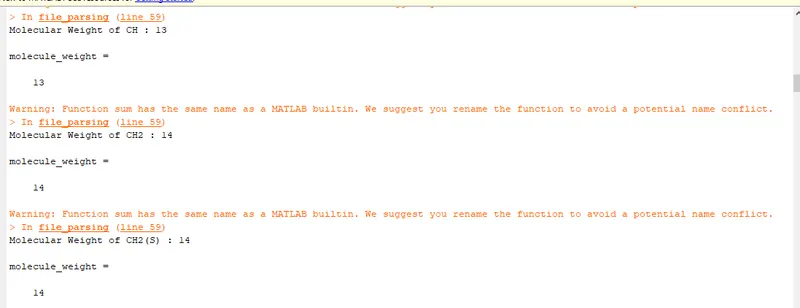
• 53-seperate folder for each species:

• WORKSPACE RESILTS:

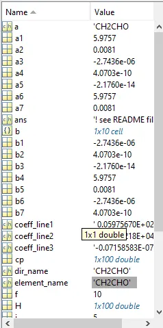
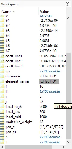
• A detailed report to describe my logic for the above code.
  • The code starts with a comment using the command “%”.

• Then, write the commands “clear all”,” close all” and “clc” to clear the workspace, close other programs, and clear the command window screen.

• To open the given data file, I’m using the command “fopen()” and stored in the desired variable as shown in the code.

• Now, to read the starting five (5) lines I’m generating “for loop” with the range of 1:5 and use the command “fgetl(f)l” to read those lines.

• Then if we observe the given data files, as we have read the first five lines of this given data. That means out of 218 lines 5 lines are read.

• As per data, the pattern is clearly every 1 to 4 lines each element species is given. That means we have 53 species and each species contains 4 lines.

• Using the above pattern, I’m storing the element species from the first line of 53 species.

• After that, I’m getting out the data of local low temperature, local high temperature, and local mid temperature.

• Now assigning the coefficients a1,a2,a3,a4,a5,a7,b1,b2,b3,b4,b5,b6,b7 value as shown in the code.

• Then, I’m creating a new directory on the default library to store all 53 species plots in a separate folder.

• Using the command ” cd('C:\Users\admin\Documents\MATLAB')

• dir_name = element_name;

  mkdir(dir_name);

  cd(element_name)”

• After that, I’m defining the “T” using the command “linspace(local_temp,local_high,1000)” having a size of 1000.

• Then, I’m calling out the function ”therm_prop” and assigning the value as [cp,H,S], where cp is specific heat, H is enthalpy, and S is entropy.

• Also, the function “molecular_weight” and assigning this value as molecule_name.

• Now, I’m plotting this value as shown in the code and storing all three figure in separate species folder using the command “savesas(figure,’filename.format’)”.

• So, in this manner, the whole code work and give the results.