Air Standard Cycle

CHALLENGE:5

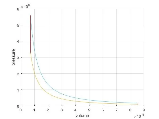
• Write code that can solve an otto cycle and make plots for it.

%Writing the code for solving an otto cycle and make plots for it.

clear all
close all
clc

%input 
gamma = 1.4
 %state variables
 p1 =101325
 t1 = 500
 t3 = 2300
 % engine parameters 
 bore = 0.1;
 stroke = 0.1;
 con_rod = 0.15;
 cr = 12;

 % calculating the swept volume
 v_swept = (pi/4)*bore^2*stroke;

 %calculating the clearance volume
 v_clearance = v_swept/(cr-1);

%for 1-2 isentropic compression process
 v1 = v_swept+v_clearance
 v2 = v_clearance

 p2 = p1*(v1/v2)^gamma
 t2 =p2*v2*t1/(p1*v1)

constant_c =p1*v1^gamma;
v_compression = engine_kinematics(bore,stroke,con_rod,cr,180,0);
 p_compression = constant_c./v_compression.^gamma;

 
%data for 2-3 constant volume heat addition process
v3=v2
p3 = p2*t3/t2


%data for 3-4 isentropic expansion process
v4 = v1

p4 = p3*(v3/v4)^gamma

constant_c =p3*v3^gamma;
v_expansion = engine_kinematics(bore,stroke,con_rod,cr,180,0);
 p_expansion = constant_c./v_expansion.^gamma;

% to draw the "p-v diagram" 
hold on
plot(v1,p1,'color','r')
xlabel('volume')
ylabel('pressure')

plot(v2,p2)
plot(v_compression,p_compression)

plot(v3,p3)
plot(v4,p4)
plot(v_expansion,p_expansion)
plot([v1 v4],[p1 p4],'color', 'r')
plot([v2 v3],[p2 p3],'color', 'r')

grid on

• The above code is incomplete because we are using the "function" command,so to run the above code we should also require that "source function" code which can be given as,

  function [V] = engine_kinematics(bore,stroke,con_rod,cr,start_crank,end_crank)
  
  a = stroke/2;
  R =con_rod/a;
  v_swept = (pi/4)*bore^2*stroke;
   v_clearance = v_swept/(cr-1);
  
   theta = linspace(start_crank,end_crank,100);
    term1 = 0.5*(cr-1);
    term2 = R+1- cosd(theta);
    term3 = (R.^2- sind(theta).^2).^0.5;
  
    V = (1+term1*(term2-term3))*v_clearance
  
  end
  

• NOTE:

USE THE BOTH GIVEN CODE TO GET RESULT.

• RESULT:

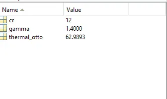
• The output of the thermal efficiency of the engine:

clear all
close all
clc

%input 
gamma = 1.4
 cr = 12
% To calculate the thermal efficiency of otto cycle
thermal_otto = (1-1/cr^(gamma-1))*100

• RESULT:

• Step-wise explanation of the above codes.
• Firstly, I started the code with a comment using the '%' command.
• Defining the needed variables for calculation.
• Using the theoretically based calculation for the otto cycle, I'm going to find out all the required terms needed for plotting the "p-v diagram" of the otto cycle.
• As shown in all three above codes.
• To draw the curve for a "p-v diagram" of the otto cycle, I'm going to create another program where I'm going to find actual compression done by the piston at IDC(inner death center) and ODC(outer death center).
• Defining all terms to get the volume compression value(refer to the second code).
• Using the "function" command for callout this code in the first code.
• To plot p-v diagram for otto cycle(used code),
• hold on

  plot(v1,p1,'color','r')

  xlabel('volume')

  ylabel('pressure')

  plot(v2,p2)

  plot(v_compression,p_compression)

  plot(v3,p3)

  plot(v4,p4)

  plot(v_expansion,p_expansion)

  plot([v1 v4],[p1 p4],'color', 'r')

  plot([v2 v3],[p2 p3],'color', 'r')

  grid on
• So, finally, we get a p-v diagram for the otto cycle.
• Now, we have to find the thermal efficiency of the Otto cycle.
• For this, I'm creating a new program(refer to third code).
• Defining the required variables and getting the thermal efficiency of the Otto cycle(in percentage).
• So, this was the explanation of the three codes used by me.