Week 3 - Solving second order ODEs

SOLVING SECOND ORDER ODE'S EQUATION USING MATLAB

• write a program that solves the following ODE:

%writing the program to solve the above ode's equation


clear all
close all
clc

%inputing the data for solving the given equation
b=0.05;
g=9.81;
l=1;
m=0.1;

theta_0 =[0;3];

tspan = linspace(0,20,500);

[t, results] = ode45(@(t,theta)ode_func(t,theta,b,g,l,m),tspan,theta_0);
plot(t,results(:,1))
hold on
 plot(t,results(:,2))
xlabel('plot')
ylabel('time')

• The insider code in the above program can be given as.

function [dtheta_dt] = ode_func(t,theta,b,g,l,m)

theta1 = theta(1)
theta2 = theta(2)

dtheta1_dt = theta2;

dtheta2_dt = -(b/m)*theta2 - (g/l)*sin(theta1);

dtheta_dt = [dtheta1_dt; dtheta2_dt]

end

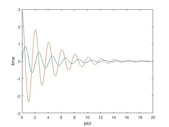
• Result:

• Step-wise explanation of the above code.
• I'm starting my code with comments using the "%" command.
• Then I assign the value as per the given data.
• After assigning the data, I'm going to use the "ode45()" command to solve the above-given equation.
• The "ode45" command is used for integrates the system of differential equations y'=f(t,y) from t0 to tf with initial conditions y0.
• After that finally, I plot the values as per the given code to get the above result.
• So in this way, the above ode's equation gets solved using Matlab.

• "ODE45" SYNTAX:
• The command "ode45()" is used for integrates the system of differential equations of second-order differential equations.
• Syntax for ode45 can be given as,

ode45(ode_function(),t_span,y0)

where t_span and y0 are limits for integration.

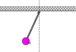
• Using the above information, let's animate the motion of the pendulum using MaTlab, as shown in the below figure.

%writing the program to animate simple pendulum oscillation

clear all
close all
clc

%inputing the data for animation creation of simple pendulum oscillation
b=0.05;
g=9.81;
l=1;
m=0.1;
x0 =1;
y0=1;

theta_0 =[0;3];

tspan = linspace(0,20,500);

[t, results] = ode45(@(t,theta)ode_func(t,theta,b,g,l,m),tspan,theta_0);
theta = results(:,1);

%program for animation creation
ctr=1;

for i = 1:length(theta)
    
    Theta = theta(i);
    x1 = 1- l*sin(Theta);
    y1 = 1- cos(theta(i));

    plot([0 2], [1 1],'lineWidth',52,'color','r')
    hold on
    plot([x0 x1], [y0 y1],'lineWidth',3,'color','b')
    plot([x1 x1],[y1 y1],'o','markersize',30,'color','g')
    hold off
    pause(0.02)
    axis([0 2 -0.5 1.5])
    M(ctr) = getframe(gcf);

    ctr=ctr+1;
end

%for creating video files and saving the data

movie(M)
videofile = VideoWriter('Simple pendulum.avi','Uncompressed AVI');
open(videofile)
writeVideo(videofile,M)
close(videofile)

• RESULT:

YOUTUBE VIDEO LINK:

https://youtu.be/AHZHBOeHZU0

• Step-wise explanation of the above code.
• I'm starting my code with comments using the "%" command.
• Then I assign the value as per the given data.
• Then, using the "for loop" command assigning the different values to 'Theta' in the above program.

• for better animation, i'm using the "ctr=1...ct=ct+1" command for contouring frame.
• for making animation video, i'm using,