Project 1 - Parsing NASA thermodynamic data
NASA came up with polynomials that can be used to evaluate thermodynamic properties such as Cp, H and S. They have also documented the co-efficients that are required to evaluate these polynomials for 1000+ species.
To guide you we have broken down the problem into meaningful bits that you can work on individually.
Question 1. Write a function that extracts the 14 co-efficients and calculates the enthalpy, entropy and specific heats for all the species in the data file. You will be reading this file NASA thermodynamic data(Tip: use fopen and fgetl). The formulae are shown below.
Note given: Here R is the universal gas constant, T is the temeprature

The FIRST 7 coefficients are HIGH-temperature coefficients and the SECOND 7 coefficients are LOW-temperature coefficients. Also use the LOCAL TEMPERATURE RANGES which is unique for each individual species, not the GLOBAL TEMPERATURE RANGE.
Solution:
The thermodynamic properties associated with the thermodynamic data with different coefficient polynomials and species are as follows:
- Specific heat
- Entropy and
- Enthalpy
Specific heat: It is defined as the quantity of heat required to raise the temperature of one gram of a substance by one Celsius degree. The units of specific heat are usually calories or joules per gram per Celsius degree.

R is the universal gas constant, as given in the question, the first 7 coefficients are high temperature (i.e more than 1000K) and the second 7 coefficients are low temperature (below 1000K).
Specific heat function can be defined as follows:
%Specific heat function
function cp=specificheat(a1,a2,a3,a4,a5,a8,a9,a10,a11,a12,temp,R,global_mid_temperature)
if (temp<=global_mid_temperature) %conditional statement to evaluate the specific heat
    cp=R.*(a8+(a9*temp) +(a10*(temp).^2)+(a11*(temp).^3)+(a12*(temp).^4));
else
    cp=R.*(a1+(a2*temp) +(a3*(temp).^2)+(a4*(temp).^3)+(a5*(temp).^4));
end
end
Entropy:
It is defined as the measure of a system’s thermal energy per unit temperature that is unavailable for doing useful work. Because work is obtained from ordered molecular motion, the amount of entropy is also a measure of the molecular disorder, or randomness, of a system.

%entropy function
function S=Entropy_S(a1,a2,a3,a4,a5,a7,a8,a9,a10,a11,a12,a14,temp,R,global_mid_temperature);
if temp <= global_mid_temperature
    S=R.*(a8.*log(temp) +(a9.*temp)+(a10*((temp).^2)/2)+(a11*((temp).^3)/3)+(a12*((temp).^4)/4)+a14);
else
    S=R.*(a1.*log(temp) +(a2.*temp)+(a3*((temp).^2)/2)+(a4*((temp).^3)/3)+(a5*((temp).^4)/4)+a7);
end
end
Enthalpy: It is defined as the sum of the internal energy(U) and the product of pressure(P) and volume(V).
Enthalpy H can be written as, H = U + pV
Where, H = Enthalpy of the system
U = Internal energy of the system
p = Pressure of the system
V = Volume of the system

%Enthalpy funtion
function H=enthalpy(a1,a2,a3,a4,a5,a6,a8,a9,a10,a11,a12,a13,temp,R,global_mid_temperature);
if (temp<=global_mid_temperature)
    H=R.*temp.*(a8+((a9*temp)/2)+(a10*(temp).^2)/3)+((a11*(temp).^3)/4)+((a12*(temp).^4)/5)+((a13./temp));
else
    H=R.*temp.*(a1+((a2*temp)/2)+(a3*(temp).^2)/3)+((a4*(temp).^3)/4)+((a5*(temp).^4)/5)+((a6./temp));
end
end
From the NASA thermodynamic data file provided, the lines starting with ! mark can be ignored since it is a comment line.

Below are the code to ignore the comment line from the file provided.
%To skip all the comment lines starting with "!"
for i=1:3
    ignore=fgetl(f1)
end
Molecular Weight: The molecular weight ( molar mass ) of any gas is the mass of one particle of that gas multiplied by Avogadro's number (6.02 x 10²³)
function  M=molecularweight(species);
atomic_variables=['H','O' ,'N' ,'A', 'C'] %Various atomic names
variable_weight=[1.008,15.999,14.007,39.948,12.011] %weights of the atomic elements
M=0;%initial value of molecular weight
for i=1:length(species)
    for j=1:length(atomic_variables)
        if strcmpi(species(i),atomic_variables(j))
            M=M+variable_weight(j);
            position=j;
        end
    end
    n=str2num(species(i));
    if n>1
        M=M+variable_weight(position)*(n-1);
    end
end
fprintf('molecular weight of %s',species)
fprintf('%f',M)
disp(' ')
end
Main Program that takes the "THERMO.dat" file as an input and generate Cp, H and S plots and also the code that includes the function link, plot and coefficients are as follows:
Program Description:
Step 1: %cleaning command script- close all will closes all open MATLAB figure window, clear all will clear all data stored to a variable and the command clc will clear the command window.
Step 2: fopen(filename) opens the file, filename , for binary read access, and returns an integer file identifier equal to or greater than 3. After which the temperature is read from the header provided in the thermodynamic data file.
Step 3: str2num was used to Convert character array or string to numeric array and temperature ranges were provided between global_low_temperature and global_high_temperature of 1000 values in between them.
Step 4: After initializing and assigning all variables, the coefficient of polynomial of the thermodynamic properties were determined by first identifying the location of E in the values and providing the formulae before and after the location of E. This will enable us to identify various coefficients such as a1, a2, a3, a4,a5,a6, a7, a8, a9,a10, a11, a12, a13, and a14.
clear all
close all
clc
%Opening and reading the data file provided
f1=fopen('THERMO.dat','r')
fgetl(f1);
%To read the temperature from heaer
globaltemperature=fgetl(f1)
A=strsplit(globaltemperature);%splitting
%Conversion of string to numbers
global_low_temperature=str2num(A{2});
global_mid_temperature=str2num(A{3});
global_high_temperature=str2num(A{4});
%roviding ranges of temperature
temp=linspace(global_low_temperature,global_high_temperature,1000);
%Universal gas constant
R=8.314;

%To skip all the comment lines starting with "!"
for i=1:3
    ignore=fgetl(f1)
end

for k=1:53
    tline=fgetl(f1)
    B=strsplit(tline,' ')
    species=(B{1})
  L1=fgetl(f1);
  a=findstr(L1,'E')
  %Finding first 7 coefficients - high temperature
  a1=L1(1:a(1)+3)
  a1=str2num(a1)
  a2=L1(a(1)+4:a(2)+3)
  a2=str2num(a2)
  a3=L1(a(2)+4:a(3)+3)
  a3=str2num(a3)
  a4=L1(a(3)+4:a(4)+3)
  a4=str2num(a4)
  a5=L1(a(4)+4:a(5)+3)
  a5=str2num(a5)

  L2=fgetl(f1);
  b=findstr(L2,'E')
  a6=L2(1:b(1)+3)
  a6=str2num(a6)
  a7=L2(b(1)+4:b(2)+3)
  a7=str2num(a7)
  %Extracting second 7 coefficients - low temperatures
  a8=L2(b(2)+4:b(3)+3);
  a8=str2num(a8);
  a9=L2(b(3)+4:b(4)+3);
  a9=str2num(a9);
  a10=L2(b(4)+4:b(5)+3);
  a10=str2num(a10)

  L3=fgetl(f1)
  c=findstr(L3,'E');
  a11=L3(1:c(1)+3);
  a11=str2num(a11);
  a12=L3(c(1)+4:c(2)+3);
  a12=str2num(a12);
  a13=L3(c(2)+4:c(3)+3);
  a13=str2num(a13);
  a14=L3(c(3)+4:c(4)+3);
  a14=str2num(a14);

  %calculate specific heat
  cp=specificheat(a1,a2,a3,a4,a5,a8,a9,a10,a11,a12,temp,R,global_mid_temperature);
  %calculate entropy
  S=Entropy_S(a1,a2,a3,a4,a5,a7,a8,a9,a10,a11,a12,a14,temp,R,global_mid_temperature);
  %calculate Enthalpy
  H=enthalpy(a1,a2,a3,a4,a5,a6,a8,a9,a10,a11,a12,a13,temp,R,global_mid_temperature);
  %Calculate molecular weight
  M(i)=molecularweight(species);

  molecularlist=fopen('molecularweight.txt','a+');
  fprintf(molecularlist,'molecular weight of %s is %d \n', species,M);
  fclose(molecularlist);
  %for saving the plots in a folder for each species
  cur_dir=pwd;
  mkdir(species);
  cd(species);
  %Plotting Specific heat and temperatures
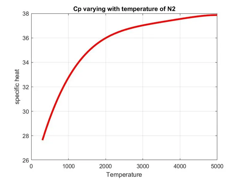
  figure(1)
  plot(temp,cp,'LineWidth',3,'color','r')
  xlabel('Temperature')%Providing x axis label
  ylabel('specific heat')%Providing Y axis label
  title(sprintf('Cp varying with temperature of %s',species));%providing title tothe plot for each species
  grid on
  saveas(figure(1),'specific heat.jpg');%Saving the figure
  %Plotting Entropy and temperatures
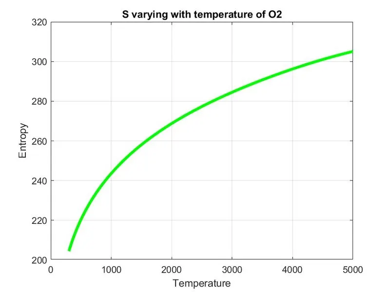
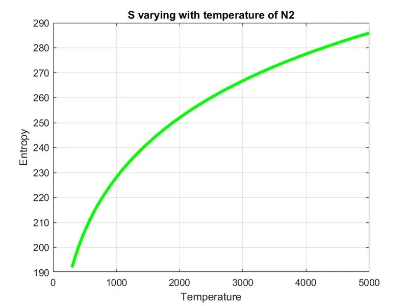
  figure(2)
  plot(temp,S,'LineWidth',3,'color','g')
  xlabel('Temperature') %Providing x axis label
  ylabel('Entropy')%Providing Y axis label
  title(sprintf('S varying with temperature of %s',species));%providing title tothe plot for each species
  grid on
  saveas(figure(2),'Entropy.jpg');%Saving the figure
  %Plotting Enthalpy and temperatures
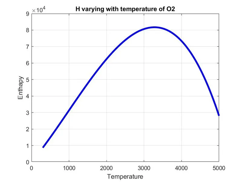
  figure(3)
  plot(temp,H,'LineWidth',3,'Color','b')
  xlabel('Temperature')%Providing x axis label
  ylabel('Enthapy')%Providing Y axis label
  title(sprintf('H varying with temperature of %s',species));%providing title tothe plot for each species
  grid on
  saveas(figure(3),'Enthalpy.jpg');%Saving the figure
  cd(cur_dir);
  %Molecular weight
  M=molecularweight(species)
end
Step 5: Now a funciton is provided for three different properties such as specific heat, entropy and enthalpy to call out the input arguments and evaluate the value to further plot the properties against the temperature ranges.
coefficient a1 to a7 is high_Temperature and coefficients a8-a14 is low_temperature coefficients.
Step 6: Figure command is used to generate the plot with xlabel and ylabel to provide labels to the graphical representation of x-axis and y-axis.
Step 7: Molecular weight is denoted as M and the atomic_variables provided are H O C N A. After providing the variables_weight foreach element deoted above and by initally initializing the variable M=0, we can create a loop condition which runs for different species. strcmp was used to compare the strings. We can use the scanf command to include the name of different species in the title.
Step 8: To save te plots, saveas command was used for each plot figures.
2. Calculate the molecular weight of each species and display it in the command window.
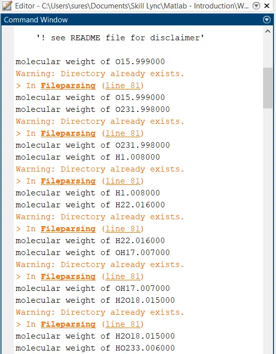
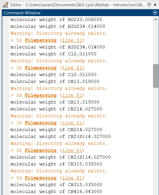
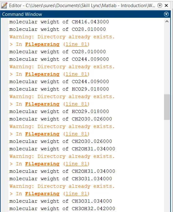
The above details are just for reference. Seperate text file was created to fetch the molecular weight of each species.
Link to refer the text document of molecular weight:
https://drive.google.com/file/d/1Pbu1ksaeFuiySiXCLtRrHATTAFsnGb-q/view?usp=sharing
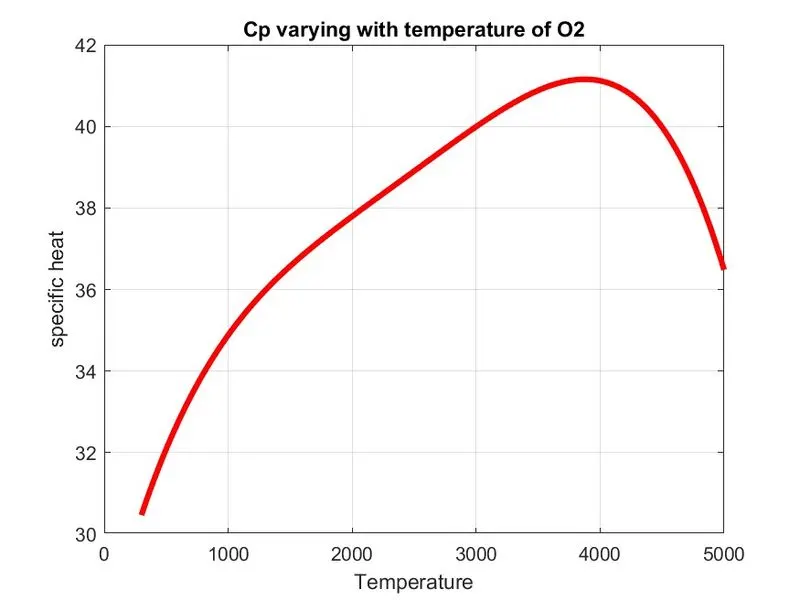
3. Plot the Cp, Enthalpy and Entropy for the local temperature range (low temperature : high temperature) specific for each species.
Plots for o2, N2 and Co2 species:
Plot 1: Variation of cp,H and S for O2 Species:
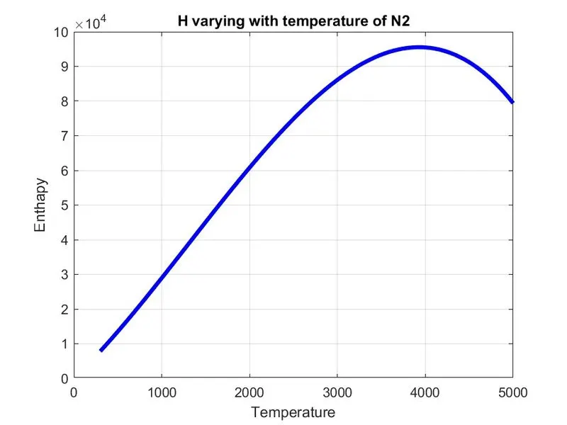
Plot 2: Variation of cp,H and S for N2 Species:
Plot 3: Variation of cp,H and S for CO2 Species:
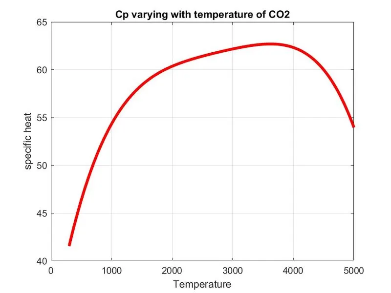
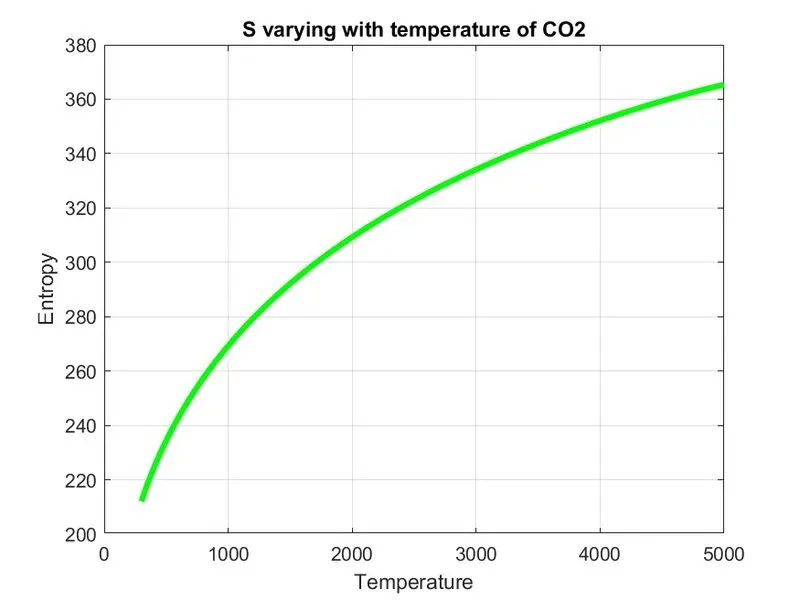
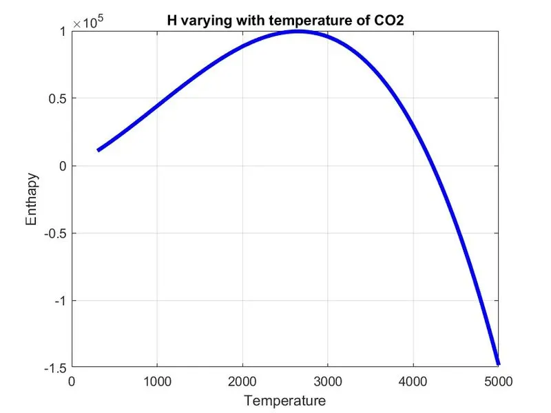
Output description: All the coefficients were evaluated from the thermodynamic data file provided with which the plot were produced to understand the variation of cp, H and S over different temperature ranges between the global_low_temperature and global_high_temperature.
4. Save the plots as images with appropriate names and dump them in separate folders for each species with suitable name. All these should be generated automatically.
Links to the species folder and plots:
https://drive.google.com/drive/folders/1Ox-_-gAwDqyasRe1Gc7cMhExcGELpb6F?usp=sharing

Errors obtained:
Error 1: Typo error: length was entered with spelling mistake.
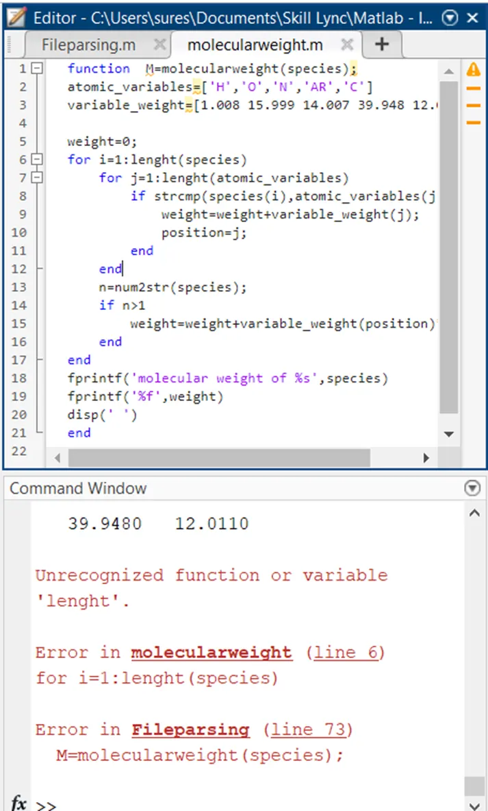
Steps to rectify the above error: Changed the spelling of length from lenght to length.
Error 2: Syntax error and character mistake. instead of typing n>1, there was a character mistake where i entered "?"
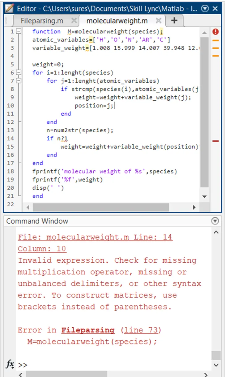
Steps to rectify the above error: Changed the character from "?" to ">". This further produced correct result.
References:
Entropy description
https://www.britannica.com/science/entropy-physics
str2num description (MATLAB)
https://in.mathworks.com/help/matlab/ref/str2num.html
fopen link (MATLAB)
https://in.mathworks.com/help/matlab/ref/fopen.html
strcmp description