Project 1 - Parsing NASA thermodynamic data
Aim :- To evaluate thermodynamic properties such as Cp,H and S. They have also documented the co-efficients that are required to evaluate these polynomials for 1000+ species.
Objective :-
Writing a function that extracts the 14 co-efficients and claculates the enthalpy, entropy and specific heats for all the species In the data file. By reading this file NASA Thermodynamic data file.(Tip: use fopen and fget). The formulae are are shown below:
Here R is the universal gas constant, T is the temeprature
he FIRST 7 coefficients are HIGH-temperature coefficients and the SECOND 7 coefficients are LOW-temperature coefficients.
Also use the LOCAL TEMPERATURE RANGES which is unique for each individual species, not the GLOBAL TEMPERATURE RANGE.
- Calculate the molecular weight of each species and display it in the command window.
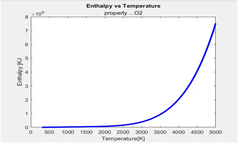
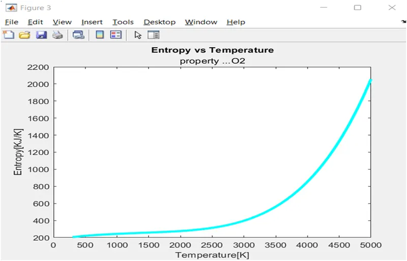
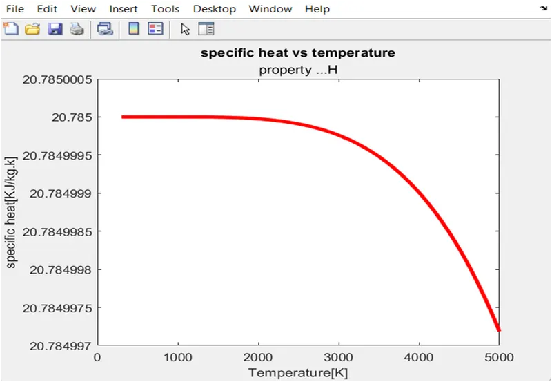
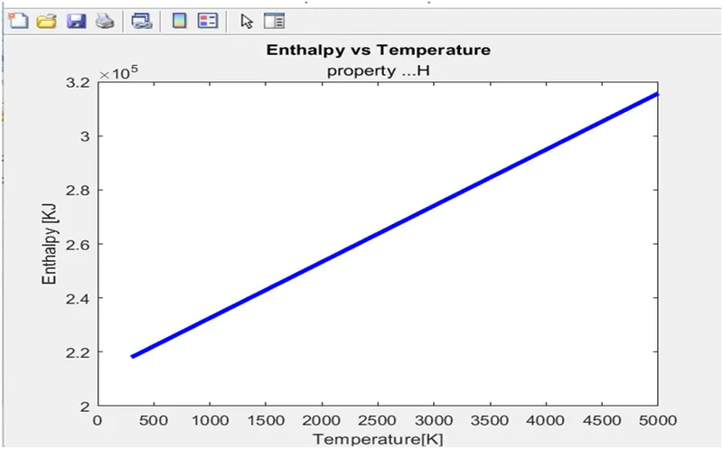
- Plot the Cp, Enthalpy and Entropy for the local temperature range (low temperature : high temperature) specific for each species.
- Save the plots as images with appropriate names and dump them in separate folders for each species with suitable name. All these should be generated automatically.
Theory :
Specicific Heat :-
specific heat, the quantity of heat required to raise the temperature of one gram of a substance by one Celsius degree. The units of specific heat are usually calories or joules per gram per Celsius degree.
Enthalpy :-
Enthalpy is the measurement of energy in a thermodynamic system. The quantity of enthalpy equals to the total content of heat of a system, equivalent to the system’s internal energy plus the product of volume and pressure. When a process begins at constant pressure, the evolved heat (either absorbed or released) equals the change in enthalpy. Enthalpy change is the sum of internal energy denoted by U and product of volume and Pressure, denoted by PV, expressed in the following manner .
H=U+PV
Entropy :-
Entropy is one of the important concepts that students need to understand clearly while studying Chemistry and Physics. More significantly, entropy can be defined in several ways and thus can be applied in various stages or instances such as in a thermodynamic stage, cosmology, and even in economics. The concept of entropy basically talks about the spontaneous changes that occur in the everyday phenomenon or the tendency of the universe towards disorder.
Apart from being just a scientific concept entropy is often described as a measurable physical property that is most commonly associated with uncertainty. However, the term is also used in different fields ranging from classical thermodynamics, statistical physics and even information theory. In addition to its applications in Physics and Chemistry, it’s applied in biological systems and their relation to life, sociology, weather science and climate change as well as to quantify the transmission of information in telecommunication.
File parsing :-
File parsing means reading a file from the outer folder inside the matlab or extracting the value of a folder provided extracting the value inside the folder. The name parse refers in matlab reading a function, script or internal code inside the memory. Some of the common commands used are (fopen,fgetl,fgets, etc.)
Explanation :-
- Getting the heading of the file.
- The given program will get the header of the file wich start with clear all close all clc.
- The command fopen will used for reading the thermodynamic data.
- The fgetl command returns the next line of the specified file, removing the newline chraracters.
- If the file is nonempty, then fgetreturns tline as a character vector.
- If the file is empty and contains only the end-of-file marker, then fgetreturns tline as a numeric value -1.
Code :-
%% NASA Thermodynamic Data and calculating the molicular weight
clear all
close all
clc
diary Results_NASA_Thermo_Data.txt;
% Getting the header info
f1 = fopen('THERMO.dat','r');
header = fgetl(f1);
Getting the global temperature :
- The global temperature info is stored in string so we use the command str2double so that it returns the value in {} as a string.
- Which gives us the cell array. From wich we can get the global temperature value.
- For skipping the next three comments we use fgetl command.
Code :-
% Getting the temperature data
global_temp = fgetl(f1);
x = strsplit(global_temp);
global_temp_low = str2double(x{2});
global_temp_mid = str2double(x{3});
global_temp_high = str2double(x{4});
fgetl(f1);
fgetl(f1);
fgetl(f1);
Getting the temperature info of individual species :
- Species name is store in length of 6 for that I used line (1:6) matlab will give me the value and so on for getting the low_temp value which is on 49 to 55th location I used the command line1(49:55) matlab will get me the value. As well for heigher temp and mid temp.
- Here in this section I have use the terms local_temp which show I am targetting the temperature of the species.
- And then converting to the string by using again str2double command. With giving temperature name low_temp,high_temp,mid_temp.
Code :-
% getting the line
line1 = fgetl(f1);
species_name = line1(1:6);
% getting local temp
local_temp1 = line1(49:55);
low_temp = str2double(local_temp1);
local_temp2 = line1(58:65);
mid_temp = str2double(local_temp2);
local_temp3 = line1(68:75);
high_temp = str2double(local_temp3);
Extracting the co-efficient values :
- In order to extract co-efficient value I got the lines by fgetl command and marked the lines as line2,line3,line4 and I use these line to extract the co-efficient.
- By using the line2,line3,line4 I will try to separate the co-efficient taking a constant E and I will use the command strfind to find E, which lies at same position at every length.
- So I target E as the extractor of my co-efficient plus the extra numbers. And same for all the 14 coefficient.
- And to converted string I have used the command str2double.
Code :-
%% Extracting the main coefficients from the data
% co-effient
line2 = fgetl(f1);
line3 = fgetl(f1);
line4 = fgetl(f1);
a = strfind(line2,'E');
b = strfind(line3,'E');
c = strfind(line4,'E');
% For low temp
a1 = str2double(line2(1:a(1)+3));
a2 = str2double(line2(a(1)+4:a(2)+3));
a3 = str2double(line2(a(2)+4:a(3)+3));
a4 = str2double(line2(a(3)+4:a(4)+3));
a5 = str2double(line2(a(4)+4:a(5)+3));
a6 = str2double(line3(1:b(2)+3));
a7 = str2double(line3(b(1)+4:b(2)+3));
a8 = str2double(line3(b(2)+4:b(3)+3));
a9 = str2double(line3(b(3)+4:b(4)+3));
a10 = str2double(line3(b(4)+4:b(5)+3));
a11 = str2double(line4(1:c(1)+3));
a12 = str2double(line4(c(1)+4:c(2)+3));
a13 = str2double(line4(c(2)+4:c(3)+3));
a14 = str2double(line4(c(3)+4:c(4)+3));
Specific Heat function :-
- Here I have used the same formula as mention above to calculate the cp,h and s value.
- For loop is for repeating these condition for all three at once cp,h and s.
- If loop is used here because there are condition for all applied for finding value all 7 co-efficient of higher temperature and value of 7 co-efficient of lower temperature.
Code :-
function [cp, h, s] = coeff(a1,a2,a3,a4,a5,a6,a7,a8,a9,a10,a12,a13,a14,T)
% Given conditions
R = 8.314;
for j = 1:length(T)
if T(j)<300
cp = (a1+a2.*T+a3.*T.^2+a4.*T.^3+a5.*T.^4).*R;
h =(a1+(a2.*T)./2+(a3.*T.*T^2)./3+(a4.*T.^3)./4+(a5.*T.^4)./5+(a6./T)).*R.*T;
s = (a1.*log(T)+a2.*T+(a3.*T.^2)./2+(a4.*T.^3)./3+(a5.*T.^4)./4+a7).*R;
else
cp = (a8+a9.*T+a10.*T.^2+a11.*T.^3+a12.*T.^4).*R;
h = (a8+(a9.*T)./2+(a10.*T.^2)./3+(a11.*T.^3)./4+(a12.*T.^4)./5+(a13./T)).*R.*T;
s = (a8.*log(T)+a9.*T+(a10.*T.^2)./2+(a11.*T.^3)./3+(a12.*T.^4)./4+a14).*R;
end
end
end
Molecular Weight function :-
- Hence we can see the thermodynamic data contain 5 species that are oxygen, carbon,nitrogen, Hydrogen, Argon.
- These are named as elements and are stored in array.
- Where as their atomic masses are stored in atomic mass array,
- Here I have used for loop so that the process is to be repeated for each and every species.
- Strcmp command is used to compare the elements and corresponding atomic mass,
- And the molecular weight is stored in mol_wt.
- And the molecular weight is calculated.
- Now I have to pass this function to the main code,
Code :-
function [molecular_weight_cal] = mole_wt(species_name)
elements = {'H','N','O','C','A'};
atomic_mass = [1 14 16 12 40];
mol_wt = 0;
for i =1:length(species_name)
for j= 1:length(elements)
if strcmp(species_name(i),elements(j))
mol_wt = mol_wt+atomic_mass(j);
m=j;
end
end
s = str2double(species_name(i));
if s > 1
mol_wt = mol_wt+(atomic_mass(m)*(s-1));
end
end
molecular_weight_cal = mol_wt
fprintf('molecular_weight_cal of %s:-',species_name)
fprintf(' ')
fprintf('amu')
fprintf('n')
end
Creating a folder:
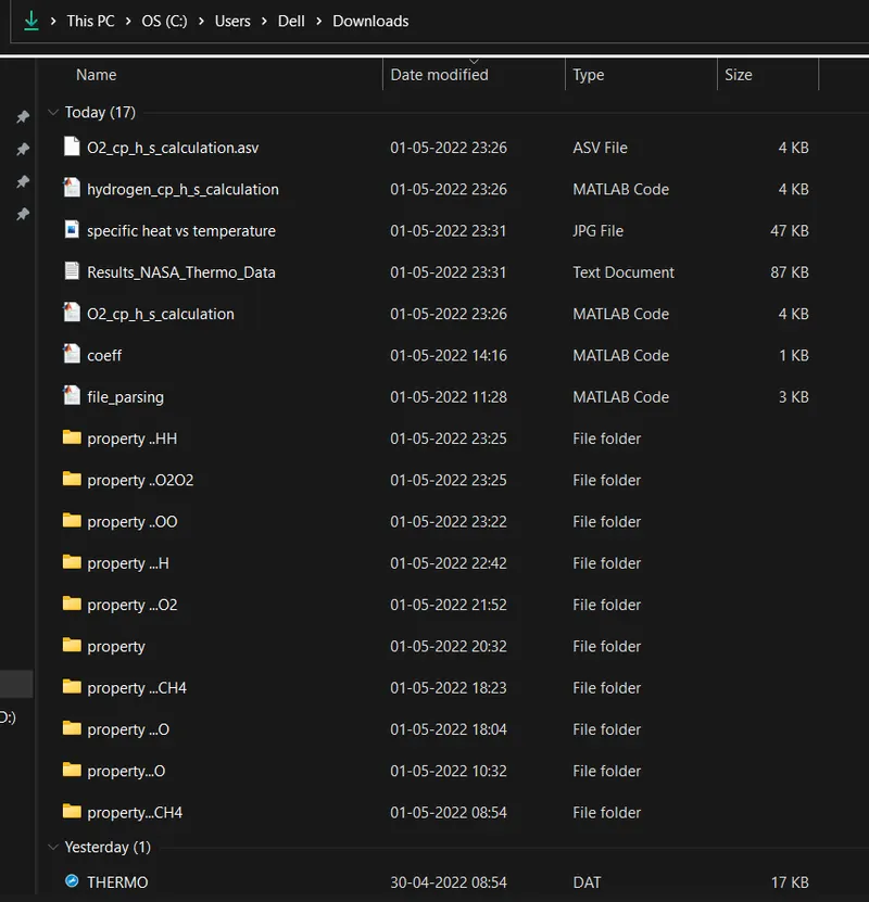
- Inorder to create a folder I have used the command mkdir which allows matlab to create a new folder to store the species data.
- Strcat command is used to concatenate a string to identify the name of the folder.
- Pwd command is used to identify the nature of the folder. For example.txt.file etc.
Code:-
% Creaing a folder 'SPECIES' to save all the species_name
species_name = strcat('property...',species_name);
mkdir(species_name);
file = pwd;
Plotting Graph :-
- Plot the graph between cp and temperature, enthalpy vs temperature, entropy vs temperature.
- Saving the graph by using fulfill command which store the entire data generated into the folder
- Gcf command is used to handle current figure.
- Cd command is used to define path to the folder where the data has to be stored.
Code :-
% plotting between Temperature and specific heat
figure(1)
plot(T,cp,'linewidth',3,'Color','r')
title('specific heat vs temperature',species_name);
xlabel('Temperature[K]')
ylabel('Enthalpy[KJ]')
f =fullfile(species_name);
% ploting between Temperature and enthalpy
figure(2)
plot(T,h,'LineWidth',3,'color','b')
title('Enthalpy vs Temperature',species_name);
xlabel('Temperature[K]')
ylabel('Enthalpy [KJ')
f = fullfile(species_name);
cd(f);
saveas(gcf,[pwd '/enthalpy bs temperature.jpg']);
cd(file)
% Plotting temperature vs entropy
figure(3)
plot(T,s,'LineWidth',3,'Color','c');
title('Entropy vs Temperature',species_name)
xlabel('Temperature[K]')
ylabel('Entropy[KJ/K]')
f = fullfile(species_name);
cd(f)
saveas(gcf,[pwd '/entropy vs temperature.jpg']);
cd(file);
Main Code :-
%% NASA Thermodynamic Data and calculating the molicular weight
clear all
close all
clc
diary Results_NASA_Thermo_Data.txt;
% Getting the header info
f1 = fopen('THERMO.dat','r');
header = fgetl(f1);
% Getting the temperature data
global_temp = fgetl(f1);
x = strsplit(global_temp);
global_temp_low = str2double(x{2});
global_temp_mid = str2double(x{3});
global_temp_high = str2double(x{4});
fgetl(f1);
fgetl(f1);
fgetl(f1);
% getting the line
line1 = fgetl(f1);
species_name = line1(1:6);
% getting local temp
local_temp1 = line1(49:55);
low_temp = str2double(local_temp1);
local_temp2 = line1(58:65);
mid_temp = str2double(local_temp2);
local_temp3 = line1(68:75);
high_temp = str2double(local_temp3);
%% Extracting the main coefficients from the data
% co-effient
line2 = fgetl(f1);
line3 = fgetl(f1);
line4 = fgetl(f1);
a = strfind(line2,'E');
b = strfind(line3,'E');
c = strfind(line4,'E');
% For low temp
a1 = str2double(line2(1:a(1)+3));
a2 = str2double(line2(a(1)+4:a(2)+3));
a3 = str2double(line2(a(2)+4:a(3)+3));
a4 = str2double(line2(a(3)+4:a(4)+3));
a5 = str2double(line2(a(4)+4:a(5)+3));
a6 = str2double(line3(1:b(2)+3));
a7 = str2double(line3(b(1)+4:b(2)+3));
a8 = str2double(line3(b(2)+4:b(3)+3));
a9 = str2double(line3(b(3)+4:b(4)+3));
a10 = str2double(line3(b(4)+4:b(5)+3));
a11 = str2double(line4(1:c(1)+3));
a12 = str2double(line4(c(1)+4:c(2)+3));
a13 = str2double(line4(c(2)+4:c(3)+3));
a14 = str2double(line4(c(3)+4:c(4)+3));
% Creaing a folder 'SPECIES' to save all the species_name
species_name = strcat('property ...',species_name);
mkdir(species_name);
file = pwd;
% Applying universal gas constant
R = 8.314;
T = linspace(global_temp_low,global_temp_high,500);
% calculation of cp (specific heat)
[cp,h,s] = coeff(a1,a2,a3,a4,a5,a6,a7,a8,a9,a10,a11,a12,a13,a14,T); %% ploting the graph
% ploting the graph
% plotting between Temperature and specific heat
figure(1)
plot(T,cp,'linewidth',3,'Color','r')
title('specific heat vs temperature',species_name);
xlabel('Temperature[K]')
ylabel('specific heat[KJ/kg.k]')
f =fullfile(species_name);
saveas(gcf,[pwd '/specific heat vs temperature.jpg']);
cd(file);
% ploting between Temperature and enthalpy
figure(2)
plot(T,h,'LineWidth',3,'color','b')
title('Enthalpy vs Temperature',species_name);
xlabel('Temperature[K]')
ylabel('Enthalpy [KJ')
f = fullfile(species_name);
cd(f);
saveas(gcf,[pwd '/enthalpy bs temperature.jpg']);
cd(file)
% Plotting temperature vs entropy
figure(3)
plot(T,s,'LineWidth',3,'Color','c');
title('Entropy vs Temperature',species_name)
xlabel('Temperature[K]')
ylabel('Entropy[KJ/K]')
f = fullfile(species_name);
cd(f)
saveas(gcf,[pwd '/entropy vs temperature.jpg']);
cd(file);
molecular_weight_cal = mole_wt(species_name);
k = sprintf('%s mole-wt = %f',species_name);molecular_weight_cal;
disp(k);
function [molecular_weight_cal] = mole_wt(species_name)
elements = {'H','N','O','C','A'};
atomic_mass = [1 14 16 12 40];
mol_wt = 0;
for i =1:length(species_name)
for j= 1:length(elements)
if strcmp(species_name(i),elements(j))
mol_wt = mol_wt+atomic_mass(j);
m=j;
end
end
s = str2double(species_name(i));
if s > 1
mol_wt = mol_wt+(atomic_mass(m)*(s-1));
end
end
molecular_weight_cal = mol_wt;
fprintf('molecular_weight_cal of %s:-',species_name)
fprintf(' ')
fprintf('amu')
fprintf('n')
end
Results :-
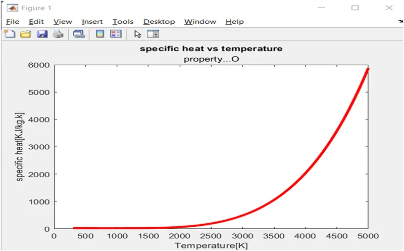
1 . cp vs temperature ‘o’
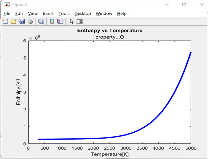
- Enthalpy vs Temperature 'o'
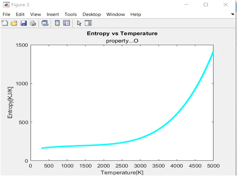
3.entropy vs temperature 'o'
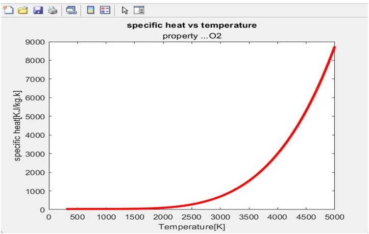
1 Specific Heat vs temperature 'O2'
2 Enthalpy vs temperature…O2
3Entropy vs temperature … O2
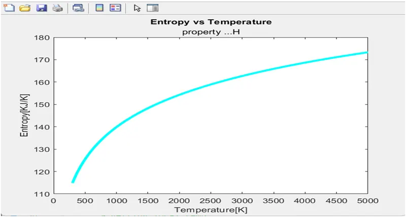
1 specific heat vs temperature hydrogen
2 Enthalpy vs temperature hydrogen
3 entropy vs Temperature for Hydrogen
Calculated molicular weight :-
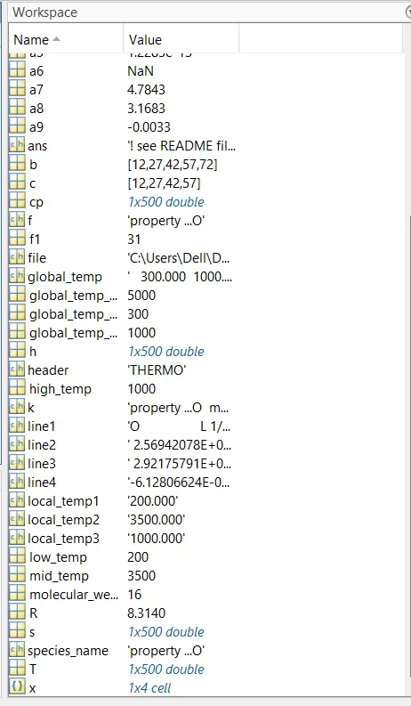
molecular_weight_cal of property ...O:- amunproperty ...O mole-wt = 16
molecular_weight_cal of property ...O2:- amunproperty ...O2mole-wt =32
molecular_weight_cal of property ...H:- amunproperty ...H mole-wt =1
Workspace window showing result value
Folder created for speciese
Errors Occurs and rectified :-
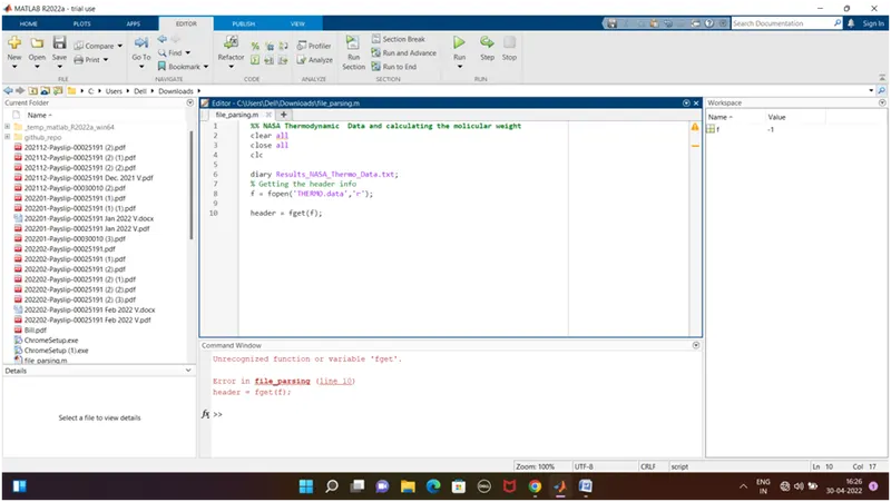
- dat file not in current folder. So to avoid this error file export in current folder.
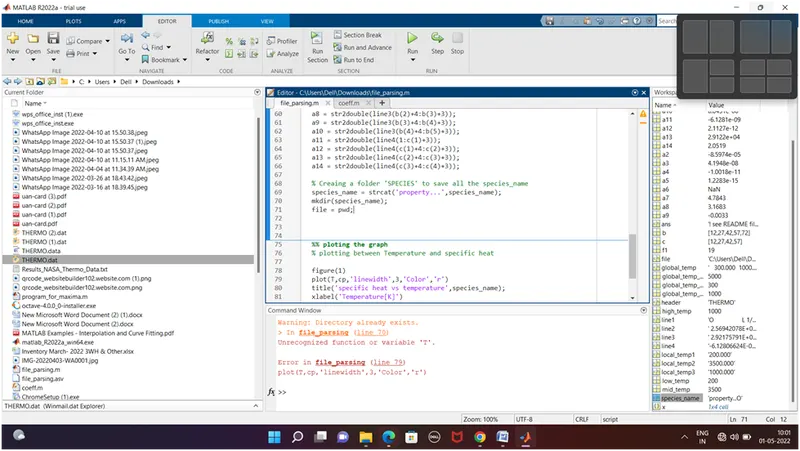
Unrecognised function of T error so define the value of T as R taking universal gas constant
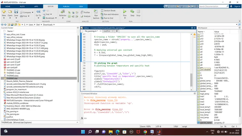
Unrecognised function of cp error calculate value of cp,h,s
Also some cyntax error is also occurs for new functions wich are rectified immediatly.
Conclusion :-
- The thermodynamic data has been parsed, and thermodynamic data has been calculated and plotted for each species.
- It has been clearly seen that the data of cp,h ad s vary at different temperature range from low temperature to high temperature to high temperature at each compound
- Hence we have calculated the molicular weight of diffent species and stored the data using file parsing technique.
Referances :-
https://www.britannica.com/science/entropy-physics
You tube
https://skill-lync.com/student-projects/project-1-parsing-nasa-thermodynamic-data-862