Project - Parsing NASA Thermodynamic Data

Project on Parsing NASA Thermodynamic data

Aim: To write a program in Matlab to parse the NASA thermodynamic data file, extract values from it and calculate different thermodynamic properties for various species.

Objectives:

1) To write a function that extracts the 14 co-efficients and calculates the enthalpy, entropy and specific heats for all the species in the data file.

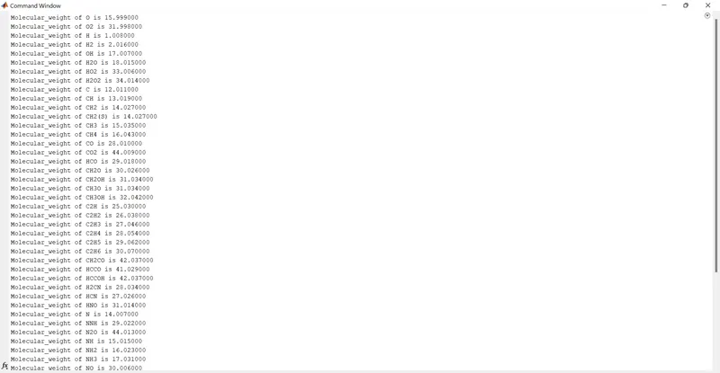
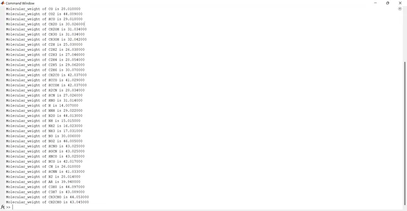
2) To calculate the molecular weight of each species and display it in the command window.

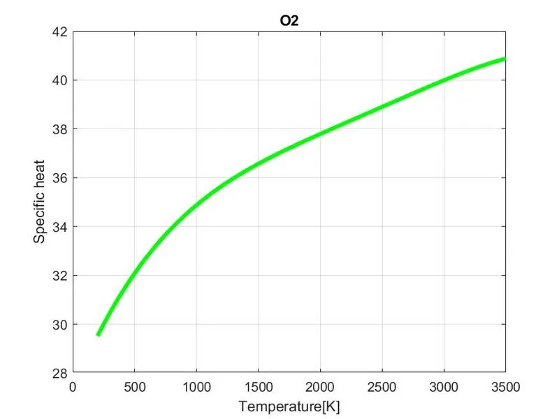
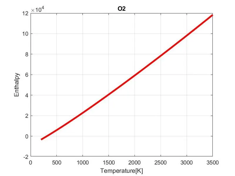
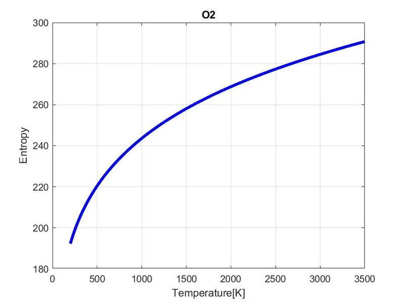
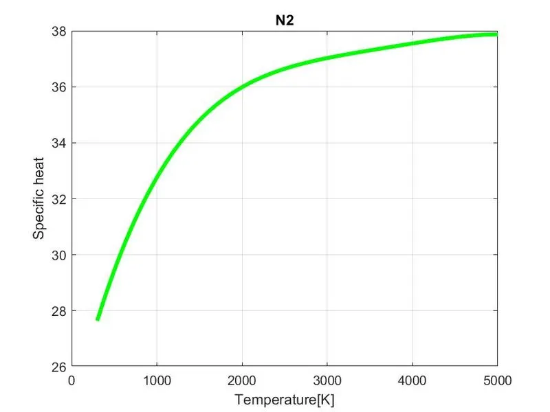
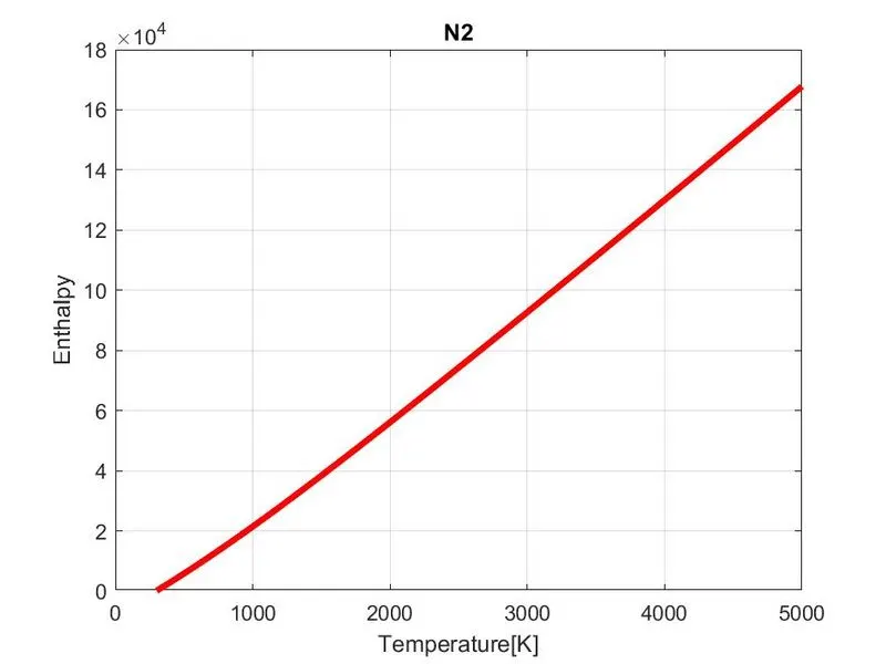
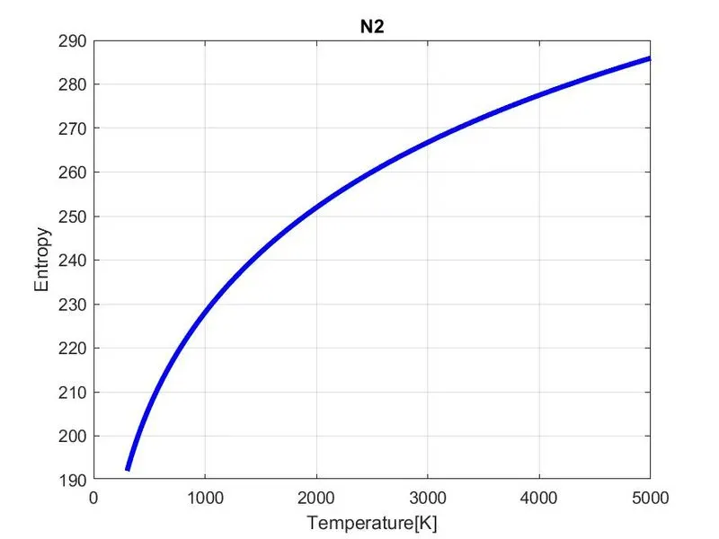
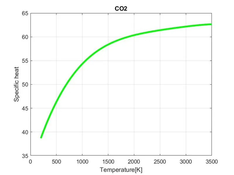
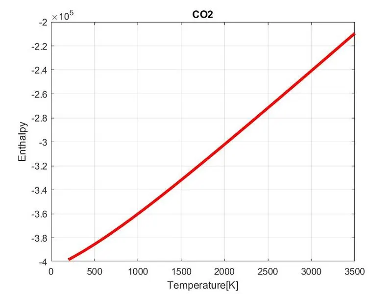
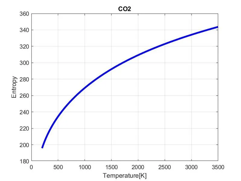
3) To plot the Cp, Enthalpy and Entropy for the local temperature range (low temperature: high temperature) specific for each species.

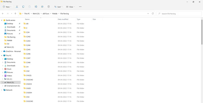
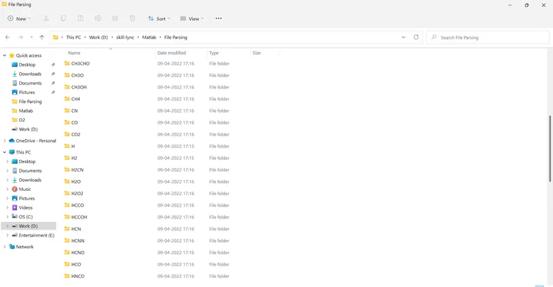
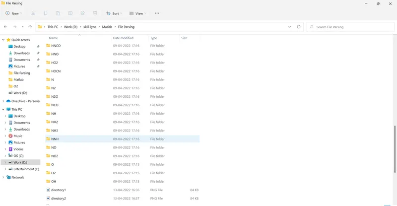
4) To save the plots as images with appropriate names and dump them in separate folders for each species with suitable name. All these should be generated automatically.

What is File Parsing?

Displayed above is the dictionary meaning of parsing. On the same lines, file parsing in Matlab is nothing but the extraction of data from a given file and resolving it into its components. The same data can be made use of in our program; with or without converting it into a different datatype. In our challenge we have been provided the NASA data file to work upon.

NASA data file

NASA came up with polynomials that can be used to evaluate thermodynamic properties such as Cp, H and S. They have also documented the co-efficients that are required to evaluate these polynomials for 1000+ species. In our case we have 53 such species which are various chemical compounds. 14 temperature coefficients, of which first seven are high temperature coefficients while next seven are low temperature coefficients. Also we have the global and local low, mid and high temperatures. The equations for various thermodynamic properties are:

where,

Cp= Specific heat

H=Enthalpy

S=Entropy

T=Temperature

R= Universal gas constant

a=All the ‘a’ values represent temperature coefficients (for our case a1-a7 are high temperature coefficients and a8-a14 are low temperature coefficients)

Understanding the code

MATLAB Script link:

https://drive.google.com/drive/folders/1dn0G9IMlWbw2UKolYN-bEK8OGyejBXL1?usp=sharing

The data file

THERMO
   300.000  1000.000  5000.000
! GRI-Mech Version 3.0 Thermodynamics released 7/30/99
! NASA Polynomial format for CHEMKIN-II
! see README file for disclaimer
O                 L 1/90O   1               G   200.000  3500.000  1000.000    1
 2.56942078E+00-8.59741137E-05 4.19484589E-08-1.00177799E-11 1.22833691E-15    2
 2.92175791E+04 4.78433864E+00 3.16826710E+00-3.27931884E-03 6.64306396E-06    3
-6.12806624E-09 2.11265971E-12 2.91222592E+04 2.05193346E+00                   4
O2                TPIS89O   2               G   200.000  3500.000  1000.000    1
 3.28253784E+00 1.48308754E-03-7.57966669E-07 2.09470555E-10-2.16717794E-14    2
-1.08845772E+03 5.45323129E+00 3.78245636E+00-2.99673416E-03 9.84730201E-06    3
-9.68129509E-09 3.24372837E-12-1.06394356E+03 3.65767573E+00                   4
H                 L 7/88H   1               G   200.000  3500.000  1000.000    1
 2.50000001E+00-2.30842973E-11 1.61561948E-14-4.73515235E-18 4.98197357E-22    2
 2.54736599E+04-4.46682914E-01 2.50000000E+00 7.05332819E-13-1.99591964E-15    3
 2.30081632E-18-9.27732332E-22 2.54736599E+04-4.46682853E-01                   4
H2                TPIS78H   2               G   200.000  3500.000  1000.000    1
 3.33727920E+00-4.94024731E-05 4.99456778E-07-1.79566394E-10 2.00255376E-14    2
-9.50158922E+02-3.20502331E+00 2.34433112E+00 7.98052075E-03-1.94781510E-05    3
 2.01572094E-08-7.37611761E-12-9.17935173E+02 6.83010238E-01                   4
OH                RUS 78O   1H   1          G   200.000  3500.000  1000.000    1
 3.09288767E+00 5.48429716E-04 1.26505228E-07-8.79461556E-11 1.17412376E-14    2
 3.85865700E+03 4.47669610E+00 3.99201543E+00-2.40131752E-03 4.61793841E-06    3
-3.88113333E-09 1.36411470E-12 3.61508056E+03-1.03925458E-01                   4
H2O               L 8/89H   2O   1          G   200.000  3500.000  1000.000    1
 3.03399249E+00 2.17691804E-03-1.64072518E-07-9.70419870E-11 1.68200992E-14    2
-3.00042971E+04 4.96677010E+00 4.19864056E+00-2.03643410E-03 6.52040211E-06    3
-5.48797062E-09 1.77197817E-12-3.02937267E+04-8.49032208E-01                   4
HO2               L 5/89H   1O   2          G   200.000  3500.000  1000.000    1
 4.01721090E+00 2.23982013E-03-6.33658150E-07 1.14246370E-10-1.07908535E-14    2
 1.11856713E+02 3.78510215E+00 4.30179801E+00-4.74912051E-03 2.11582891E-05    3
-2.42763894E-08 9.29225124E-12 2.94808040E+02 3.71666245E+00                   4
H2O2              L 7/88H   2O   2          G   200.000  3500.000  1000.000    1
 4.16500285E+00 4.90831694E-03-1.90139225E-06 3.71185986E-10-2.87908305E-14    2
-1.78617877E+04 2.91615662E+00 4.27611269E+00-5.42822417E-04 1.67335701E-05    3
-2.15770813E-08 8.62454363E-12-1.77025821E+04 3.43505074E+00                   4
C                 L11/88C   1               G   200.000  3500.000  1000.000    1
 2.49266888E+00 4.79889284E-05-7.24335020E-08 3.74291029E-11-4.87277893E-15    2
 8.54512953E+04 4.80150373E+00 2.55423955E+00-3.21537724E-04 7.33792245E-07    3
-7.32234889E-10 2.66521446E-13 8.54438832E+04 4.53130848E+00                   4
CH                TPIS79C   1H   1          G   200.000  3500.000  1000.000    1
 2.87846473E+00 9.70913681E-04 1.44445655E-07-1.30687849E-10 1.76079383E-14    2
 7.10124364E+04 5.48497999E+00 3.48981665E+00 3.23835541E-04-1.68899065E-06    3
 3.16217327E-09-1.40609067E-12 7.07972934E+04 2.08401108E+00                   4
CH2               L S/93C   1H   2          G   200.000  3500.000  1000.000    1
 2.87410113E+00 3.65639292E-03-1.40894597E-06 2.60179549E-10-1.87727567E-14    2
 4.62636040E+04 6.17119324E+00 3.76267867E+00 9.68872143E-04 2.79489841E-06    3
-3.85091153E-09 1.68741719E-12 4.60040401E+04 1.56253185E+00                   4
CH2(S)            L S/93C   1H   2          G   200.000  3500.000  1000.000    1
 2.29203842E+00 4.65588637E-03-2.01191947E-06 4.17906000E-10-3.39716365E-14    2
 5.09259997E+04 8.62650169E+00 4.19860411E+00-2.36661419E-03 8.23296220E-06    3
-6.68815981E-09 1.94314737E-12 5.04968163E+04-7.69118967E-01                   4
CH3               L11/89C   1H   3          G   200.000  3500.000  1000.000    1
 2.28571772E+00 7.23990037E-03-2.98714348E-06 5.95684644E-10-4.67154394E-14    2
 1.67755843E+04 8.48007179E+00 3.67359040E+00 2.01095175E-03 5.73021856E-06    3
-6.87117425E-09 2.54385734E-12 1.64449988E+04 1.60456433E+00                   4
CH4               L 8/88C   1H   4          G   200.000  3500.000  1000.000    1
 7.48514950E-02 1.33909467E-02-5.73285809E-06 1.22292535E-09-1.01815230E-13    2
-9.46834459E+03 1.84373180E+01 5.14987613E+00-1.36709788E-02 4.91800599E-05    3
-4.84743026E-08 1.66693956E-11-1.02466476E+04-4.64130376E+00                   4
CO                TPIS79C   1O   1          G   200.000  3500.000  1000.000    1
 2.71518561E+00 2.06252743E-03-9.98825771E-07 2.30053008E-10-2.03647716E-14    2
-1.41518724E+04 7.81868772E+00 3.57953347E+00-6.10353680E-04 1.01681433E-06    3
 9.07005884E-10-9.04424499E-13-1.43440860E+04 3.50840928E+00                   4
CO2               L 7/88C   1O   2          G   200.000  3500.000  1000.000    1
 3.85746029E+00 4.41437026E-03-2.21481404E-06 5.23490188E-10-4.72084164E-14    2
-4.87591660E+04 2.27163806E+00 2.35677352E+00 8.98459677E-03-7.12356269E-06    3
 2.45919022E-09-1.43699548E-13-4.83719697E+04 9.90105222E+00                   4
HCO               L12/89H   1C   1O   1     G   200.000  3500.000  1000.000    1
 2.77217438E+00 4.95695526E-03-2.48445613E-06 5.89161778E-10-5.33508711E-14    2
 4.01191815E+03 9.79834492E+00 4.22118584E+00-3.24392532E-03 1.37799446E-05    3
-1.33144093E-08 4.33768865E-12 3.83956496E+03 3.39437243E+00                   4
CH2O              L 8/88H   2C   1O   1     G   200.000  3500.000  1000.000    1
 1.76069008E+00 9.20000082E-03-4.42258813E-06 1.00641212E-09-8.83855640E-14    2
-1.39958323E+04 1.36563230E+01 4.79372315E+00-9.90833369E-03 3.73220008E-05    3
-3.79285261E-08 1.31772652E-11-1.43089567E+04 6.02812900E-01                   4
CH2OH             GUNL93C   1H   3O   1     G   200.000  3500.000  1000.000    1
 3.69266569E+00 8.64576797E-03-3.75101120E-06 7.87234636E-10-6.48554201E-14    2
-3.24250627E+03 5.81043215E+00 3.86388918E+00 5.59672304E-03 5.93271791E-06    3
-1.04532012E-08 4.36967278E-12-3.19391367E+03 5.47302243E+00                   4
CH3O              121686C   1H   3O   1     G   300.00   3000.00   1000.000    1
 0.03770799E+02 0.07871497E-01-0.02656384E-04 0.03944431E-08-0.02112616E-12    2
 0.12783252E+03 0.02929575E+02 0.02106204E+02 0.07216595E-01 0.05338472E-04    3
-0.07377636E-07 0.02075610E-10 0.09786011E+04 0.13152177E+02                   4
CH3OH             L 8/88C   1H   4O   1     G   200.000  3500.000  1000.000    1
 1.78970791E+00 1.40938292E-02-6.36500835E-06 1.38171085E-09-1.17060220E-13    2
-2.53748747E+04 1.45023623E+01 5.71539582E+00-1.52309129E-02 6.52441155E-05    3
-7.10806889E-08 2.61352698E-11-2.56427656E+04-1.50409823E+00                   4
C2H               L 1/91C   2H   1          G   200.000  3500.000  1000.000    1
 3.16780652E+00 4.75221902E-03-1.83787077E-06 3.04190252E-10-1.77232770E-14    2
 6.71210650E+04 6.63589475E+00 2.88965733E+00 1.34099611E-02-2.84769501E-05    3
 2.94791045E-08-1.09331511E-11 6.68393932E+04 6.22296438E+00                   4
C2H2              L 1/91C   2H   2          G   200.000  3500.000  1000.000    1
 4.14756964E+00 5.96166664E-03-2.37294852E-06 4.67412171E-10-3.61235213E-14    2
 2.59359992E+04-1.23028121E+00 8.08681094E-01 2.33615629E-02-3.55171815E-05    3
 2.80152437E-08-8.50072974E-12 2.64289807E+04 1.39397051E+01                   4
C2H3              L 2/92C   2H   3          G   200.000  3500.000  1000.000    1
 3.01672400E+00 1.03302292E-02-4.68082349E-06 1.01763288E-09-8.62607041E-14    2
 3.46128739E+04 7.78732378E+00 3.21246645E+00 1.51479162E-03 2.59209412E-05    3
-3.57657847E-08 1.47150873E-11 3.48598468E+04 8.51054025E+00                   4
C2H4              L 1/91C   2H   4          G   200.000  3500.000  1000.000    1
 2.03611116E+00 1.46454151E-02-6.71077915E-06 1.47222923E-09-1.25706061E-13    2
 4.93988614E+03 1.03053693E+01 3.95920148E+00-7.57052247E-03 5.70990292E-05    3
-6.91588753E-08 2.69884373E-11 5.08977593E+03 4.09733096E+00                   4
C2H5              L12/92C   2H   5          G   200.000  3500.000  1000.000    1
 1.95465642E+00 1.73972722E-02-7.98206668E-06 1.75217689E-09-1.49641576E-13    2
 1.28575200E+04 1.34624343E+01 4.30646568E+00-4.18658892E-03 4.97142807E-05    3
-5.99126606E-08 2.30509004E-11 1.28416265E+04 4.70720924E+00                   4
C2H6              L 8/88C   2H   6          G   200.000  3500.000  1000.000    1
 1.07188150E+00 2.16852677E-02-1.00256067E-05 2.21412001E-09-1.90002890E-13    2
-1.14263932E+04 1.51156107E+01 4.29142492E+00-5.50154270E-03 5.99438288E-05    3
-7.08466285E-08 2.68685771E-11-1.15222055E+04 2.66682316E+00                   4
CH2CO             L 5/90C   2H   2O   1     G   200.000  3500.000  1000.000    1
 4.51129732E+00 9.00359745E-03-4.16939635E-06 9.23345882E-10-7.94838201E-14    2
-7.55105311E+03 6.32247205E-01 2.13583630E+00 1.81188721E-02-1.73947474E-05    3
 9.34397568E-09-2.01457615E-12-7.04291804E+03 1.22156480E+01                   4
HCCO              SRIC91H   1C   2O   1     G   300.00   4000.00   1000.000    1
 0.56282058E+01 0.40853401E-02-0.15934547E-05 0.28626052E-09-0.19407832E-13    2
 0.19327215E+05-0.39302595E+01 0.22517214E+01 0.17655021E-01-0.23729101E-04    3
 0.17275759E-07-0.50664811E-11 0.20059449E+05 0.12490417E+02                   4
HCCOH              SRI91C   2O   1H   2     G   300.000  5000.000  1000.000    1
 0.59238291E+01 0.67923600E-02-0.25658564E-05 0.44987841E-09-0.29940101E-13    2
 0.72646260E+04-0.76017742E+01 0.12423733E+01 0.31072201E-01-0.50866864E-04    3
 0.43137131E-07-0.14014594E-10 0.80316143E+04 0.13874319E+02                   4
H2CN               41687H   2C   1N   1     G   300.00   4000.000  1000.000    1
 0.52097030E+01 0.29692911E-02-0.28555891E-06-0.16355500E-09 0.30432589E-13    2
 0.27677109E+05-0.44444780E+01 0.28516610E+01 0.56952331E-02 0.10711400E-05    3
-0.16226120E-08-0.23511081E-12 0.28637820E+05 0.89927511E+01                   4
HCN               GRI/98H   1C   1N   1     G   200.000  6000.000  1000.000    1
 0.38022392E+01 0.31464228E-02-0.10632185E-05 0.16619757E-09-0.97997570E-14    2
 0.14407292E+05 0.15754601E+01 0.22589886E+01 0.10051170E-01-0.13351763E-04    3
 0.10092349E-07-0.30089028E-11 0.14712633E+05 0.89164419E+01                   4
HNO               And93 H   1N   1O   1     G   200.000  6000.000  1000.000    1
 0.29792509E+01 0.34944059E-02-0.78549778E-06 0.57479594E-10-0.19335916E-15    2
 0.11750582E+05 0.86063728E+01 0.45334916E+01-0.56696171E-02 0.18473207E-04    3
-0.17137094E-07 0.55454573E-11 0.11548297E+05 0.17498417E+01                   4
N                 L 6/88N   1               G   200.000  6000.000  1000.000    1
 0.24159429E+01 0.17489065E-03-0.11902369E-06 0.30226245E-10-0.20360982E-14    2
 0.56133773E+05 0.46496096E+01 0.25000000E+01 0.00000000E+00 0.00000000E+00    3
 0.00000000E+00 0.00000000E+00 0.56104637E+05 0.41939087E+01                   4
NNH               T07/93N   2H   1          G   200.000  6000.000  1000.000    1
 0.37667544E+01 0.28915082E-02-0.10416620E-05 0.16842594E-09-0.10091896E-13    2
 0.28650697E+05 0.44705067E+01 0.43446927E+01-0.48497072E-02 0.20059459E-04    3
-0.21726464E-07 0.79469539E-11 0.28791973E+05 0.29779410E+01                   4
N2O               L 7/88N   2O   1          G   200.000  6000.000  1000.000    1
 0.48230729E+01 0.26270251E-02-0.95850874E-06 0.16000712E-09-0.97752303E-14    2
 0.80734048E+04-0.22017207E+01 0.22571502E+01 0.11304728E-01-0.13671319E-04    3
 0.96819806E-08-0.29307182E-11 0.87417744E+04 0.10757992E+02                   4
NH                And94 N   1H   1          G   200.000  6000.000  1000.000    1
 0.27836928E+01 0.13298430E-02-0.42478047E-06 0.78348501E-10-0.55044470E-14    2
 0.42120848E+05 0.57407799E+01 0.34929085E+01 0.31179198E-03-0.14890484E-05    3
 0.24816442E-08-0.10356967E-11 0.41880629E+05 0.18483278E+01                   4
NH2               And89 N   1H   2          G   200.000  6000.000  1000.000    1
 0.28347421E+01 0.32073082E-02-0.93390804E-06 0.13702953E-09-0.79206144E-14    2
 0.22171957E+05 0.65204163E+01 0.42040029E+01-0.21061385E-02 0.71068348E-05    3
-0.56115197E-08 0.16440717E-11 0.21885910E+05-0.14184248E+00                   4
NH3               J 6/77N   1H   3          G   200.000  6000.000  1000.000    1
 0.26344521E+01 0.56662560E-02-0.17278676E-05 0.23867161E-09-0.12578786E-13    2
-0.65446958E+04 0.65662928E+01 0.42860274E+01-0.46605230E-02 0.21718513E-04    3
-0.22808887E-07 0.82638046E-11-0.67417285E+04-0.62537277E+00                   4
NO                RUS 78N   1O   1          G   200.000  6000.000  1000.000    1
 0.32606056E+01 0.11911043E-02-0.42917048E-06 0.69457669E-10-0.40336099E-14    2
 0.99209746E+04 0.63693027E+01 0.42184763E+01-0.46389760E-02 0.11041022E-04    3
-0.93361354E-08 0.28035770E-11 0.98446230E+04 0.22808464E+01                   4
NO2               L 7/88N   1O   2          G   200.000  6000.000  1000.000    1
 0.48847542E+01 0.21723956E-02-0.82806906E-06 0.15747510E-09-0.10510895E-13    2
 0.23164983E+04-0.11741695E+00 0.39440312E+01-0.15854290E-02 0.16657812E-04    3
-0.20475426E-07 0.78350564E-11 0.28966179E+04 0.63119917E+01                   4
HCNO              BDEA94H   1N   1C   1O   1G   300.000  5000.000  1382.000    1
 6.59860456E+00 3.02778626E-03-1.07704346E-06 1.71666528E-10-1.01439391E-14    2
 1.79661339E+04-1.03306599E+01 2.64727989E+00 1.27505342E-02-1.04794236E-05    3
 4.41432836E-09-7.57521466E-13 1.92990252E+04 1.07332972E+01                   4
HOCN              BDEA94H   1N   1C   1O   1G   300.000  5000.000  1368.000    1
 5.89784885E+00 3.16789393E-03-1.11801064E-06 1.77243144E-10-1.04339177E-14    2
-3.70653331E+03-6.18167825E+00 3.78604952E+00 6.88667922E-03-3.21487864E-06    3
 5.17195767E-10 1.19360788E-14-2.82698400E+03 5.63292162E+00                   4
HNCO              BDEA94H   1N   1C   1O   1G   300.000  5000.000  1478.000    1
 6.22395134E+00 3.17864004E-03-1.09378755E-06 1.70735163E-10-9.95021955E-15    2
-1.66599344E+04-8.38224741E+00 3.63096317E+00 7.30282357E-03-2.28050003E-06    3
-6.61271298E-10 3.62235752E-13-1.55873636E+04 6.19457727E+00                   4
NCO               EA 93 N   1C   1O   1     G   200.000  6000.000  1000.000    1
 0.51521845E+01 0.23051761E-02-0.88033153E-06 0.14789098E-09-0.90977996E-14    2
 0.14004123E+05-0.25442660E+01 0.28269308E+01 0.88051688E-02-0.83866134E-05    3
 0.48016964E-08-0.13313595E-11 0.14682477E+05 0.95504646E+01                   4
CN                HBH92 C   1N   1          G   200.000  6000.000  1000.000    1
 0.37459805E+01 0.43450775E-04 0.29705984E-06-0.68651806E-10 0.44134173E-14    2
 0.51536188E+05 0.27867601E+01 0.36129351E+01-0.95551327E-03 0.21442977E-05    3
-0.31516323E-09-0.46430356E-12 0.51708340E+05 0.39804995E+01                   4
HCNN              SRI/94C   1N   2H   1     G   300.000  5000.000  1000.000    1
 0.58946362E+01 0.39895959E-02-0.15982380E-05 0.29249395E-09-0.20094686E-13    2
 0.53452941E+05-0.51030502E+01 0.25243194E+01 0.15960619E-01-0.18816354E-04    3
 0.12125540E-07-0.32357378E-11 0.54261984E+05 0.11675870E+02                   4
N2                121286N   2               G   300.000  5000.000  1000.000    1
 0.02926640E+02 0.14879768E-02-0.05684760E-05 0.10097038E-09-0.06753351E-13    2
-0.09227977E+04 0.05980528E+02 0.03298677E+02 0.14082404E-02-0.03963222E-04    3
 0.05641515E-07-0.02444854E-10-0.10208999E+04 0.03950372E+02                   4
AR                120186AR  1               G   300.000  5000.000  1000.000    1
 0.02500000E+02 0.00000000E+00 0.00000000E+00 0.00000000E+00 0.00000000E+00    2
-0.07453750E+04 0.04366000E+02 0.02500000E+02 0.00000000E+00 0.00000000E+00    3
 0.00000000E+00 0.00000000E+00-0.07453750E+04 0.04366000E+02                   4
C3H8              L 4/85C   3H   8          G   300.000  5000.000  1000.000    1
 0.75341368E+01 0.18872239E-01-0.62718491E-05 0.91475649E-09-0.47838069E-13    2
-0.16467516E+05-0.17892349E+02 0.93355381E+00 0.26424579E-01 0.61059727E-05    3
-0.21977499E-07 0.95149253E-11-0.13958520E+05 0.19201691E+02                   4
C3H7              L 9/84C   3H   7          G   300.000  5000.000  1000.000    1
 0.77026987E+01 0.16044203E-01-0.52833220E-05 0.76298590E-09-0.39392284E-13    2
 0.82984336E+04-0.15480180E+02 0.10515518E+01 0.25991980E-01 0.23800540E-05    3
-0.19609569E-07 0.93732470E-11 0.10631863E+05 0.21122559E+02                   4
CH3CHO            L 8/88C   2H   4O   1     G   200.000  6000.000  1000.000    1
 0.54041108E+01 0.11723059E-01-0.42263137E-05 0.68372451E-09-0.40984863E-13    2
-0.22593122E+05-0.34807917E+01 0.47294595E+01-0.31932858E-02 0.47534921E-04    3
-0.57458611E-07 0.21931112E-10-0.21572878E+05 0.41030159E+01                   4
CH2CHO            SAND86O   1H   3C   2     G   300.000  5000.000  1000.000    1
 0.05975670E+02 0.08130591E-01-0.02743624E-04 0.04070304E-08-0.02176017E-12    2
 0.04903218E+04-0.05045251E+02 0.03409062E+02 0.10738574E-01 0.01891492E-04    3
-0.07158583E-07 0.02867385E-10 0.15214766E+04 0.09558290E+02                   4
END

So, we have a data file and we need to get some information out of it. For it we will have to let Matlab know about the file first. For it, we use the ‘fopen’ function. By it, we let Matlab know about such a file in our system and let it read the contents therein. The first line of our file is a title named ‘THERMO’. We just fetch it by using the ‘fgetl’ function. Next up are the global temperature values. We fetch the line at first, split it (using ‘strsplit’) at the delimiter of space and extract the low, mid and high values of the global temperatures at 2^nd, 3^rd and 4^th positions respectively. However, we get a cell array while doing so and hence we need to use curly braces ’{}’ instead of ‘()’ while providing the location number. Also, we get the values as a string datatype, but we want them to be numbers for our use. Hence, we convert them to numerical values using the ‘num2str’ function simultaneously. Next up are 3 commented lines. We just fetch and let go of them to get to our useful information.

% Parsing NASA thermodynamic data
f=fopen('THERMO.dat','r'); %Reading the file for its content
fgetl(f); %fetching line
Tline=fgetl(f);
Tline=strsplit(Tline,' '); %Splitting the line
global_low_temp=str2num(Tline{2}); %Extracting values from line and simultaneously 
                                    converting to number from string
global_mid_temp=str2num(Tline{3});
global_high_temp=str2num(Tline{4});
for i=1:3
    fgetl(f);
end

The 6^th line and thereafter in our data file contains our main content in a pattern that is similar for all the 53 species. So, each species has 4 lines of data. The first line contains the species name and the local low, high and mid temperatures. The next 3 lines contain the 14 temperature coefficients with 5 each in the first and second line, whereas, 4 in the last one. That’s it. This is the pattern followed by the data file for all the species. So, advancing in the code, to extract this info, we create a ‘for loop’ for values ranging from 1 to 53. We fetch the first line under the variable- ‘species’. Next, we split it and store it in the ‘s’ variable. Now, we create an array for species name and store the names of the species in this by extracting the first value from the ‘s’ array. Next up are the local temperatures. Their positions are towards the end of the line. Hence, we extract them from ‘s’ by giving the location as end- value. Heading on to our next lines. The next three lines contain the temperature coefficients. So, again we fetch the second line and store it in the ‘coeff_line’ variable. Now, in all the coefficient lines there is a set pattern of data. Here, the coefficient value is expressed as,

‘(+-)a.8digitsE+2digits’

that is some integer ‘a’ in + or – followed by 8 integers after the decimal point and is raised to some power of 10 using the E+ command. So, we find the location numbers of each E in the line using the ‘strfind’ function and store it in a variable named ‘x’. Now, to extract eachcoefficient we will be specifying the location of the numbers with respect to ‘E’. For the first coefficient, we write coeff_line(1:x1+3), that is the starting value to the first location of E and 3 values after it. That makes up our first coefficient. For the second coefficient and thereafter we write coeff_line(x1+4:x2+3), that is the value of the first coefficient ends at E+3 and hence the next coefficient starts immediately after it. Therefore, we write E+4 as the starting point and E+3 as the endpoint. The same follows for other coefficients. This ends the extraction of data for our use.

%Extracting the coefficients
coeff_line1=fgetl(f);
x=strfind(coeff_line1,'E'); %Finding locations of E in the line
a1=str2num(coeff_line1(1:x(1)+3));
a2=str2num(coeff_line1(x(1)+4:x(2)+3));
a3=str2num(coeff_line1(x(2)+4:x(3)+3));
a4=str2num(coeff_line1(x(3)+4:x(4)+3));
a5=str2num(coeff_line1(x(4)+4:x(5)+3));

coeff_line2=fgetl(f);
y=strfind(coeff_line2,'E');
a6=str2num(coeff_line2(1:y(1)+3));
a7=str2num(coeff_line2(y(1)+4:y(2)+3));
a8=str2num(coeff_line2(y(2)+4:y(3)+3));
a9=str2num(coeff_line2(y(3)+4:y(4)+3));
a10=str2num(coeff_line2(y(4)+4:y(5)+3));

coeff_line3=fgetl(f);
z=strfind(coeff_line3,'E');
a11=str2num(coeff_line3(1:z(1)+3));
a12=str2num(coeff_line3(z(1)+4:z(2)+3));
a13=str2num(coeff_line3(z(2)+4:z(3)+3));
a14=str2num(coeff_line3(z(3)+4:z(4)+3));

Further, we need to calculate the thermodynamic properties based on these extracted coefficients. For it, we first define these properties as functions given by the above formulae. We then call upon these functions in our code and provide the extracted coefficients as their required inputs. Also, we have T, R and local mid temperature as inputs for these functions. Therefore, we define T as an array of temperature values using ‘linspace’ command with local low and high temperatures as the start and end values and 500 values between them. R is the universal gas constant and is given by 8.314 J/mol.K, as is known to us. Diving into the function, we have stated a condition given by the if statement; which says that, if T<= the local mid temperature then we have to use the low temperature coefficients, else the high temperature coefficients are to be made use of.

%Calculating Specific heat

function [Cp]= Specific_heat(a1,a2,a3,a4,a5,a8,a9,a10,a11,a12,T,R,local_mid_temp)
if T<=local_mid_temp
    Cp=R*(a8+(a9*T)+(a10*T.^2)+(a11*T.^3)+(a12*T.^4));
else
    Cp=R*(a1+(a2*T)+(a3*T.^2)+(a4*T.^3)+(a5*T.^4));
    
end
end


%Calculating Entropy

function [S]= Entropy_fp(a1,a2,a3,a4,a5,a7,a8,a9,a10,a11,a12,a14,T,R,local_mid_temp)
if T<=local_mid_temp
    S=R*(a8*log(T)+(a9*T)+(a10*(T.^2)/2)+(a11*(T.^3)/3)+(a12*(T.^4)/4)+a14);
    
else
    S=R*(a1*log(T)+(a2*T)+(a3*(T.^2)/2)+(a4*(T.^3)/3)+(a5*(T.^4)/4)+a7);
end
end


%Calculating Enthalpy

function [E]= Enthalpy(a1,a2,a3,a4,a5,a6,a8,a9,a10,a11,a12,a13,T,R,local_mid_temp)
if T<=local_mid_temp
    E=R*T.*(a8+(a9*(T)/2)+(a10*(T.^2)/3)+(a11*(T.^3)/4)+(a12*(T.^4)/5)+(a13./T));
else
    E=R*T.*(a1+(a2*(T)/2)+(a3*(T.^2)/3)+(a4*(T.^3)/4)+(a5*(T.^4)/5)+(a6./T));
    
end
end


%Main Code
%Additional inputs for the functions
T=linspace(local_low_temp,local_high_temp,500);
R=8.314;

%Calling the functions
Cp=Specific_heat(a1,a2,a3,a4,a5,a8,a9,a10,a11,a12,T,R,local_mid_temp);
S= Entropy_fp(a1,a2,a3,a4,a5,a7,a8,a9,a10,a11,a12,a14,T,R,local_mid_temp);
E=Enthalpy(a1,a2,a3,a4,a5,a6,a8,a9,a10,a11,a12,a13,T,R,local_mid_temp);

Having obtained all these values, we plot these properties against temperature and write a code that automatically makes different folders for each species and saves these plots in them. So, to begin with we change our current directory using the ‘cd’ command. We than make a directory for each species given by the species name using ‘mkdir’ command. Then we plot each of the properties against temperature in different figures and save them with the ‘jpg’ file extension using the ‘saveas’ command. In addition, we have been told to calculate the molecular weight of each species.

cd('D:skill-lyncMatlabFile Parsing') %Current directory
mkdir(species_name) %Making new directory with the species name
cd(species_name) % Changing current directory to the one created above
figure(1) 
plot(T,Cp,'linewidth',3,'color','g')
xlabel('Temperature[K]')
ylabel('Specific heat')
title(species_name(1:end))
grid on
saveas(figure(1),'T vs Cp.jpg') %Saving the plot

figure(2)
plot(T,S,'linewidth',3,'color','b')
xlabel('Temperature[K]')
ylabel('Entropy')
title(species_name(1:end))
grid on
saveas(figure(2),'T vs S.jpg')

figure(3)
plot(T,E,'linewidth',3,'color','r')
xlabel('Temperature[K]')
ylabel('Enthalpy')
title(species_name(1:end))
grid on
saveas(figure(3),'T vs E.jpg')
cd('D:skill-lyncMatlabFile Parsing') % Again changing directory to main directory

For it, we create a function for molecular weight. In it, we create an array carrying the atomic names of each atom required to form these species. They are ‘H’,‘C’,’O’,’N’,’Ar’. Also, we provide the corresponding atomic weights for these names in the same order in a different array. We define the molecular weight to be 0 initially. Then we begin our for loop, for 1 up to the length of species array. In it we again create a for loop for 1 up to the length of the atomic name array. Then we specify a condition given by the if statement where we compare the species name and the atomic name bit by bit. Whence, the if condition gets satisfied our molecular weight is incremented by the value corresponding to the atomic weight of the atom. We then assign the current value of the second for loop variable to a variable named ‘position’. Then, we convert our species name to a numeric value and assign it to a variable ‘n’. We then check if the value of n is greater than 1. If it is so, then the if statement is executed. Let’s understand this with an example. So if our species is O2, after the end of the second for loop our O2 will get converted to a number datatype. For the first execution of the length of species loop O will be taken as the input. At any given point in time we can’t convert O which is an alphabet to a number. Hence our second if loop is terminated. Then for the next for loop our ‘n’ would carry the value 2 which happens to be a number and now this can be used to check the condition of the if statement. As 2 is greater than 1 we enter the if statement and our molecular weight is incremented. This is for all those species, which have two or more units of a same atom in its molecule. All these values are then printed in the command window using the fprintf function.

%Calculating molecular weight

function [W]=Molecular_weight(species)
atomic_name=['H' 'C' 'O' 'N' 'Ar']; 
atomic_weight=[1.008 12.011 15.999 14.007 39.948];
W=0;
for i=1:length(species)
    for j=1:length(atomic_name)
        if strcmp(species(i),atomic_name(j)) %Comparison of 2 string functions
        W=W+atomic_weight(j);
        position=j; %Position variable equal to j variable
        end
    end
    n=str2num(species); %Converting string to number
    if n>1
        W=W+atomic_weight(position)*(n-1); %For more than 2 atoms of same name in the species
    end
end
fprintf('Molecular_weight of %s is %fn',species,W) %Printing
end


%Main Code
W=Molecular_weight(species_name); %Calling molecular weight function

end

The Entire Code

% Parsing NASA thermodynamic data
f=fopen('THERMO.dat','r'); %Reading the file for its content
fgetl(f); %fetching line
Tline=fgetl(f);
Tline=strsplit(Tline,' '); %Splitting the line
global_low_temp=str2num(Tline{2}); %Extracting values from line and simultaneously converting to number from string
global_mid_temp=str2num(Tline{3});
global_high_temp=str2num(Tline{4});
for i=1:3
    fgetl(f);
end

for j=1:53 %As there are 53 species
species=fgetl(f); 
s=strsplit(species,' ');
species_name=s{1};
%Extracting local low,mid and high temperatures
local_low_temp=str2num(s{end-3});
local_mid_temp=str2num(s{end-1});
local_high_temp=str2num(s{end-2});

%Extracting the coefficients
coeff_line1=fgetl(f);
x=strfind(coeff_line1,'E'); %Finding locations of E in the line
a1=str2num(coeff_line1(1:x(1)+3));
a2=str2num(coeff_line1(x(1)+4:x(2)+3));
a3=str2num(coeff_line1(x(2)+4:x(3)+3));
a4=str2num(coeff_line1(x(3)+4:x(4)+3));
a5=str2num(coeff_line1(x(4)+4:x(5)+3));

coeff_line2=fgetl(f);
y=strfind(coeff_line2,'E');
a6=str2num(coeff_line2(1:y(1)+3));
a7=str2num(coeff_line2(y(1)+4:y(2)+3));
a8=str2num(coeff_line2(y(2)+4:y(3)+3));
a9=str2num(coeff_line2(y(3)+4:y(4)+3));
a10=str2num(coeff_line2(y(4)+4:y(5)+3));

coeff_line3=fgetl(f);
z=strfind(coeff_line3,'E');
a11=str2num(coeff_line3(1:z(1)+3));
a12=str2num(coeff_line3(z(1)+4:z(2)+3));
a13=str2num(coeff_line3(z(2)+4:z(3)+3));
a14=str2num(coeff_line3(z(3)+4:z(4)+3));

%Additional inputs for the functions
T=linspace(local_low_temp,local_high_temp,500);
R=8.314;

%Calling the functions
Cp=Specific_heat(a1,a2,a3,a4,a5,a8,a9,a10,a11,a12,T,R,local_mid_temp);
S= Entropy_fp(a1,a2,a3,a4,a5,a7,a8,a9,a10,a11,a12,a14,T,R,local_mid_temp);
E=Enthalpy(a1,a2,a3,a4,a5,a6,a8,a9,a10,a11,a12,a13,T,R,local_mid_temp);

cd('D:skill-lyncMatlabFile Parsing') %Current directory
mkdir(species_name) %Making new directory with the species name
cd(species_name) % Changing current directory to the one created above
figure(1) 
plot(T,Cp,'linewidth',3,'color','g')
xlabel('Temperature[K]')
ylabel('Specific heat')
title(species_name(1:end))
grid on
saveas(figure(1),'T vs Cp.jpg') %Saving the plot

figure(2)
plot(T,S,'linewidth',3,'color','b')
xlabel('Temperature[K]')
ylabel('Entropy')
title(species_name(1:end))
grid on
saveas(figure(2),'T vs S.jpg')

figure(3)
plot(T,E,'linewidth',3,'color','r')
xlabel('Temperature[K]')
ylabel('Enthalpy')
title(species_name(1:end))
grid on
saveas(figure(3),'T vs E.jpg')
cd('D:skill-lyncMatlabFile Parsing') % Again changing directory to main directory

W=Molecular_weight(species_name); %Calling molecular weight function

end



%Calculating Specific heat

function [Cp]= Specific_heat(a1,a2,a3,a4,a5,a8,a9,a10,a11,a12,T,R,local_mid_temp)
if T<=local_mid_temp
    Cp=R*(a8+(a9*T)+(a10*T.^2)+(a11*T.^3)+(a12*T.^4));
else
    Cp=R*(a1+(a2*T)+(a3*T.^2)+(a4*T.^3)+(a5*T.^4));
    
end
end



%Calculating Entropy

function [S]= Entropy_fp(a1,a2,a3,a4,a5,a7,a8,a9,a10,a11,a12,a14,T,R,local_mid_temp)
if T<=local_mid_temp
    S=R*(a8*log(T)+(a9*T)+(a10*(T.^2)/2)+(a11*(T.^3)/3)+(a12*(T.^4)/4)+a14);
    
else
    S=R*(a1*log(T)+(a2*T)+(a3*(T.^2)/2)+(a4*(T.^3)/3)+(a5*(T.^4)/4)+a7);
end
end


%Calculating Enthalpy

function [E]= Enthalpy(a1,a2,a3,a4,a5,a6,a8,a9,a10,a11,a12,a13,T,R,local_mid_temp)
if T<=local_mid_temp
    E=R*T.*(a8+(a9*(T)/2)+(a10*(T.^2)/3)+(a11*(T.^3)/4)+(a12*(T.^4)/5)+(a13./T));
else
    E=R*T.*(a1+(a2*(T)/2)+(a3*(T.^2)/3)+(a4*(T.^3)/4)+(a5*(T.^4)/5)+(a6./T));
    
end
end


%Calculating molecular weight

function [W]=Molecular_weight(species)
atomic_name=['H' 'C' 'O' 'N' 'Ar']; 
atomic_weight=[1.008 12.011 15.999 14.007 39.948];
W=0;
for i=1:length(species)
    for j=1:length(atomic_name)
        if strcmp(species(i),atomic_name(j)) %Comparison of 2 string functions
        W=W+atomic_weight(j);
        position=j; %Position variable equal to j variable
        end
    end
    n=str2num(species); %Converting string to number
    if n>1
        W=W+atomic_weight(position)*(n-1); %For more than 2 atoms of same name in the species
    end
end
fprintf('Molecular_weight of %s is %fn',species,W) %Printing
end

Outputs

O2 plots

N2 plots

CO2 plots

Molecular weight values

Directories

References:

Matlab documentation

!!!Thank You!!!