Modelling an electric Car with Li-ion battery
Project goal:
To model an electric vehicle with a lithium-ion battery using different drive sources as a speed reference.
Objectives:
- Create a simple Matlab model of an electric vehicle that shows all its main components as subsystems from the electric motor to the vehicle dynamics. Analyze and estimate SOC, vehicle speed, vehicle distance traveled and total energy consumption using different driving sources.
- The analysis of all the above parameters is for FTP-75, WOT and four driving cycles given at a constant speed of 100 km at a speed of 45 km/h. The entire model is simulated by varying the relevant parameters for each subsystem, such as the DC motor, H-bridge, vehicle body, etc., to determine the dependence of the subsystem parameters on the entire MATLAB model.
- The implementation of the PI controller subsystem reduces and to some extent minimizes the deviation of the actual vehicle speed from the reference speed, which is identified as a systematic error.
Introduction:
An electric vehicle (EV) is a car powered by an electric motor instead of an internal combustion engine that burns a mixture of fuel and gas to generate power. As a result, cars are considered as a possible replacement for modern cars to solve problems such as increasing pollution, global warming, depletion of natural resources, etc. Although the concept of electric vehicles has been around for a long time, the concept of electric vehicles has attracted a lot of attention in the last decade as the carbon footprint and other environmental impacts of fuel vehicles have continued to increase.
Advantages of electric cars:
- They produce no exhaust emissions and are therefore better for the planet.
- Helps EV owners avoid more expensive charging periods
- Help support the grid integration of multiple small and large renewable energy systems.
- The electricity needed to charge an electric car costs about 40 percent less than using gasoline to drive the same distance in a vehicle of the same size. The cost is lower if you charge your electric car from a solar system or from a free charging station.
- Electric vehicles (EVs) have fewer moving parts than conventional gasoline/diesel vehicles. Repairs are relatively easy, less frequent and generally cheaper than petrol/diesel cars. All EV batteries degrade (decline in efficiency). Most automakers guarantee that EV batteries will not degrade below a certain level for about eight years. You may need to replace the battery while using the electric car.
In India, the first concrete decision to incentivize electric cars was made in 2010. The government has announced financial incentives for electric vehicle manufacturers to sell in India under a Rs 950 crore scheme approved by the Ministry of New and Renewable Energy (MNRE). India. The scheme, which has been in force since November 2010, provides relief of up to 20 percent of the manufacturer's price of vehicles, subject to a ceiling. However, later in March 2012, MNRE withdrew the subsidy scheme.
In 2013, India announced the National Electric Mobility Mission Plan (NEMMP) 2020 to drive greater transition to electric vehicles and address issues such as national energy security, vehicular pollution and growth in domestic manufacturing capacity. While the plan aims to subsidize electric cars and build supporting infrastructure, the plan remains largely on paper. Introducing the Parliament with the Union 2015-2016 2018 budget, the then finance minister Arun Jaitley announced accelerated adoption and production of electric vehicles (FAME) at an initial outlay of Rs 750 crore. The announced plan aims to provide incentives for clean fuel technology vehicles to increase their sales to 7 million by 2020.
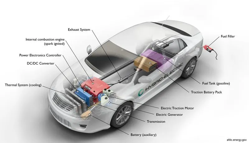
Various EV components
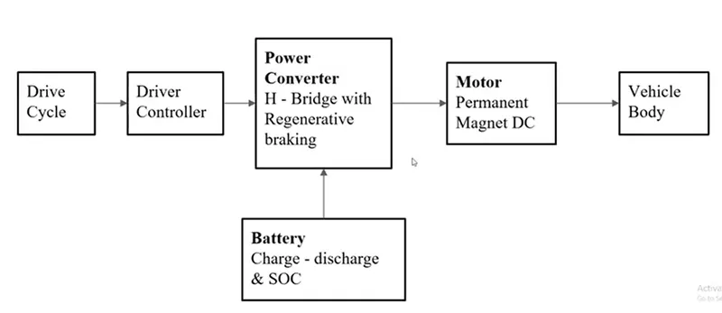
Corresponding block diagram
Another difference with electric cars is that range and efficiency are not directly related. This is due to the loss of bills; about 85% to 90% of the total power coming from the wall goes into the battery. Therefore, two concepts are used: efficiency, which can be expressed in MPGe, including charging losses, and consumption, which is the energy consumption during driving, excluding them.
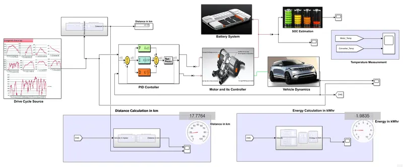
MODEL REPRESENTATION OF THE ELECTRIC CAR IN MATLAB-SIMULINK:
DESCRIPTION OF THE COMPONENTS
Drive Cycle Source Subsystem:
The Drive Cycle Subsystem Consists of the subsequent blocks that are configured as follows:
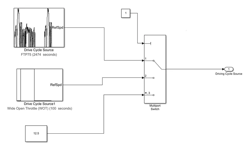
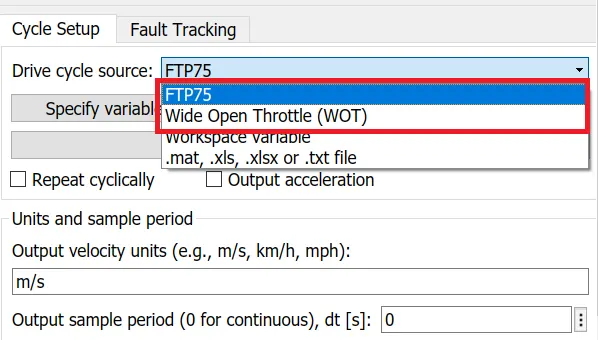
The system has 3 types of speed references, two of which are standard drive sources implemented from the "Drive Cycle Source" block, and the third is a user-defined drive cycle with a constant speed of 12.5 m/s (ie 45 km/h) giving respectively . 8000 seconds.
i) Drive Cycle Source Block:
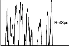
This block generates standard or user specified longitudinal drive cycles. The output of the block is the specified longitudinal velocity of the vehicle, the function is specified as:
- Predicts the engine torque and fuel consumption the vehicle needs to achieve the desired speed and acceleration for a specific shift reference.
- Generate realistic speed and shift references for closed-loop acceleration and braking commands for vehicle control and factory models.
- Explore, adapt and optimize vehicle handling, system performance and system robustness over multiple driving cycles. Drive cycles from predefined sources.
- By default, the block includes an FTP-75 drive loop.
- .mat, .xls, .xlsx or .txt files are also possible using blocks.
Select the following modes for the drive loop as shown below:
ii) Multi-port Switch:
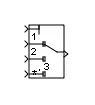
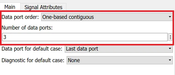
This block is used to determine which of the block's multiple inputs is sent to the output. The block makes this decision based on the value of the first input. The first input is the control input and the other inputs are the data inputs. The control input value determines which data inputs are sent to the outputs. Since this project uses 4 types of speed reference, 4 data ports are required:
PID Controller Subsystem:
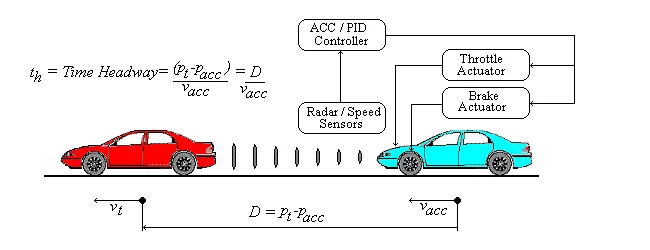
Proportional integral derivative (PID) control is the most commonly used control algorithm in industry and is widely accepted in industrial control. The popularity of PID controllers is due in part to their strong performance over a wide range of operating conditions and in part to their functional simplicity, which allows engineers to operate them simply and easily. The basic idea of a PID controller is to read the sensor and then calculate the desired output of the actuator by calculating the proportional, integral and differential response and summing these three components to calculate the output.
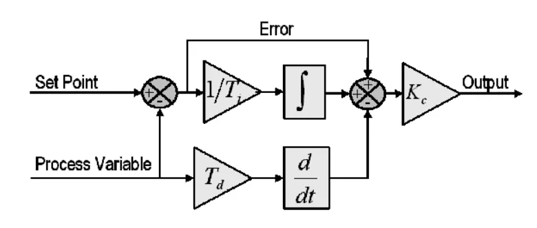
The three main responses of a PID controller are discussed below:
Proportional Response: The proportional component depends only on the difference between the setpoint and the process variable. This difference is called the error term. The proportional gain (Kc) defines the ratio of the output response to the error signal. For example, if the error word size is 10, a proportional increase of 5 will produce a proportional response of 50. In general, increasing the proportional gain will increase the response speed of the control system. However, if the proportional gain is too large, the process variable will begin to oscillate. If Kc increases further, the oscillations will become larger and the system will become unstable and may even oscillate out of control.
Integral Response: The integral sums the error term over time. The result is that even small error terms cause the integral component to grow slowly. The integral response will increase with time unless the error is zero, so the steady state error is reduced to zero. The steady state error is the difference between the process variable and the set point. When the integral action saturates the controller, but the controller does not bias the error signal to zero, a phenomenon known as integral liquidation occurs.
Derivative response: If the process variable increases rapidly, the derivative component causes the output to decrease. The differential response is proportional to the rate of change of the process variable. Increasing the derivative time (Td) parameter makes the control system more responsive to changes in the error term and increases the responsiveness of the overall control system. Most practical control systems use very small derivative times (Td) because the derivative response is very sensitive to noise in the process variable signal. If the sensor feedback signal is noisy or the speed of the control loop is too slow, the differential response can make the control system unstable.
The MATLAB model corresponding to the PID controller is shown in the figure below:
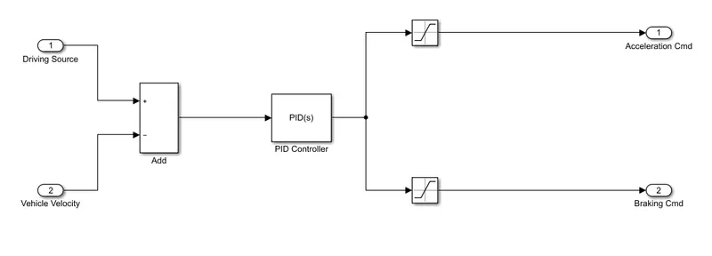
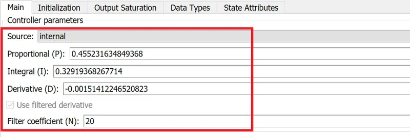
The MATLAB PID controller block performs the same function as above; The PID gain value is obtained after linearizing the device using the step-response output and tracking the error input to the PID block accordingly, the PID gain value is:
i) Saturation Block:

The saturation block produces an output signal that is the value of the input signal bounded by upper and lower saturation values. The upper and lower limits are specified by the Upper Limit and Lower Limit parameters in the command block.
Motor and its Controller Subsystem:
A motor and its controller are a device or group of devices that can coordinate the operation of a motor in a predetermined manner. Motor control may include manual or automatic devices for starting and stopping the motor, selecting forward or reverse rotation, selecting and regulating speed, regulating or limiting torque, and protecting against overload and electrical damage. Motor controls can use electromechanical switches or power electronics to regulate motor speed and direction.
This subsystem consists of blocks configured as follows:
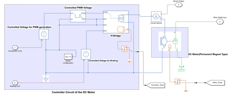
i) Controlled PWM Voltage:

This block is responsible for creating pulse width modulation (PWM) signals on the PWM and REF ports. When the pulse is low, the output voltage is zero, and when it is high, it is equal to the amplitude parameter of the output voltage. At zero, the pulse is initialized high unless the duty cycle is set to zero or the pulse delay time is greater than zero.
The required duty cycle for the electrical input port variant of the block is:
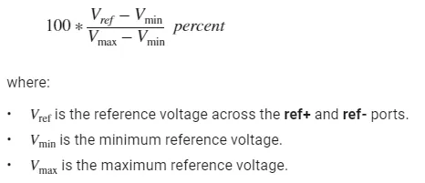
In this project, the simulation mode is chosen as average, where the output signal will be kept constant with a value corresponding to the average PWM signal. The PWM frequency is selected as 6 kHz and the output voltage range is 300 V as shown in the figure below:


(ii) H-bridge:
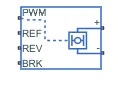
An H-bridge is a simple electronic circuit that allows us to apply voltage to a load in either direction. It is commonly used in robotic applications to control DC motors. Using H bridge we can drive DC motor clockwise or counter clockwise. This circuit is also used to generate a variable waveform in the inverter.
In MATLAB, the H-bridge module performs the same function as above, which is ultimately driven by the mid-mode controlled PWM voltage module according to the project requirements. In average mode, the PWM gate voltage divided by the PWM signal amplitude parameter determines the ratio of the on time to the PWM period. Using this relationship and load assumptions, the block applies an average voltage to the load to obtain the correct average load current. The value of the simulation mode parameter should be the same as the controlled PWM voltage and H-bridge blocks. If the REV gate voltage is greater than the inverted threshold voltage, the output voltage reverses polarity. If the voltage at the BRK gate is greater than the braking threshold voltage, the output terminal is shorted in series with a parallel combination of one bridge arm and the other bridge arm and a flyback diode.
For medium simulation mode, the load current characteristic is set to Smoothed instead of Discontinuous. On request, the H-bridge thermal gate is also enabled to monitor the change in converter temperature versus vehicle speed power.
The corresponding values for the H-Bridge parameter and the selection of the simulation mode are shown in the following figure:



(iii) DC motor (permanent magnet type):
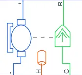
This block forms the electrical and torque characteristics of the DC motor. The assumption for this block is that there is no loss of electromagnetic energy, so the back EMF and the torque constant have the same value in SI units. Engine parameters can be specified directly or derived from idle speed and stall torque. When positive current flows from the electrical + port to the -- port, a positive torque is applied from the mechanical C port to the R port. The direction of the motor torque can be changed by changing the sign of the back EMF or the torque constant.
The motor type chosen is the permanent magnet type, so it is similar to the BLDC motor type most commonly used in electric vehicles. In this project, the thermal gate of a DC motor unit is used to simulate the effect of copper resistive losses, which convert electrical energy into heat.
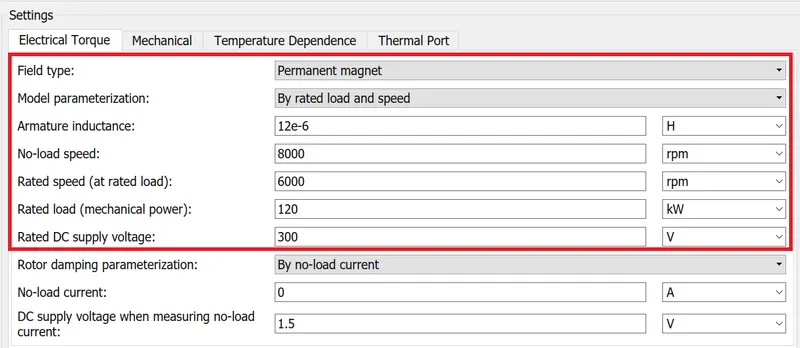
Here, the "C" port represents the engine body to be grounded using a mechanically rotating reference frame, while the "R" port represents the engine rotor, which is connected to the vehicle's dynamic transmission system. The parameter values considered by the DC motor module are shown in the figure below:


iv) Controlled Voltage Source:

The block represents an ideal voltage source strong enough to maintain the specified voltage at its output regardless of the current flowing through it. The output voltage is V = Vs, where Vs is the digital value displayed on the physical signal port.
Two sets of the power source block are required; one is needed to drive the PWM controlled voltage source and another is needed to drive the brake control of the H-bridge. The respective voltage of this block is controlled according to the acceleration command (to control the voltage source PWM) and deceleration control (to control the H-bridge braking voltage) of the longitudinal driver.
v) Current Sensor:

This block is an ideal current sensor, a device that converts the measured current in any electrical branch into a physical signal proportional to the current. The "+ve" and "-ve" connections are the electrical ports that connect the sensor to the circuit. The “I” connection is a physical signal port that outputs the current value.
The positive and negative parts of the module are connected between the H-bridge and the DC motor, while the physical port "I" is connected to the controlled power supply of the battery management system of the electric rickshaw model.
vi) Temperature Sensor:

This module measures the temperature in heat networks. No heat flows through the sensor. The physical signal port T reports the temperature difference in the sensor. The measurement is positive if the temperature at port A is higher than the temperature at port B.
Two temperature sensors are used here, one is used to measure the temperature in the H bridge and the other is used for the DC motor. The output of the sensor is taken from the physical port "T" connected to an oscilloscope to analyze the temperature profile of the motor and its inverter unit.
Vehicle Dynamic Subsystem:
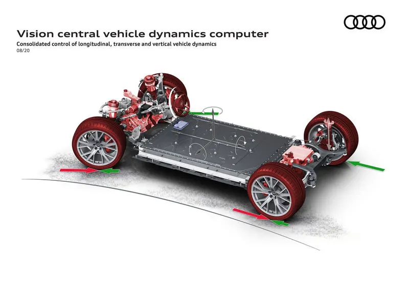
The purpose of vehicle dynamics is twofold: first, they make vehicles safer by intervening to provide support in problematic driving situations. Second, the vehicle dynamics control system can be tuned to the OEM's individual DNA. As vehicle dynamics control systems affect vehicle motion, some of these systems play an important role in achieving the goals of autonomous driving. For example, ESC applies braking in autonomous vehicles. Vehicle dynamics are constantly being improved to further improve vehicle safety and comfort. Consequently, ESC now includes various additional support functions that significantly increase the effort required for verification during development.
This subsystem consists of blocks configured as follows:
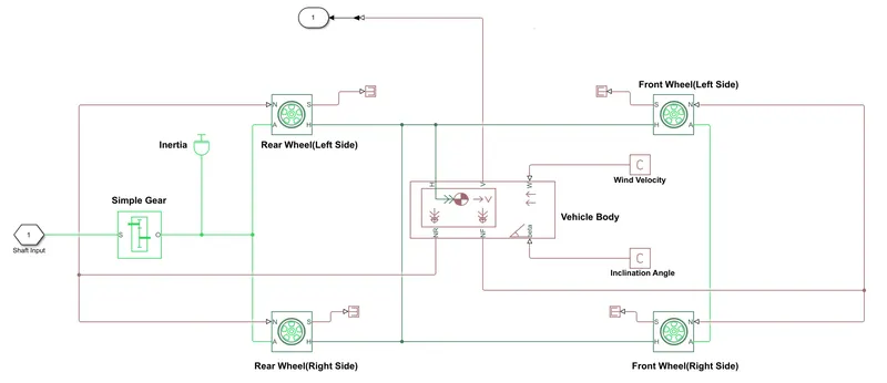
This subsystem includes blocks that are configured as follows:
i) Vehicle Body:
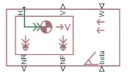
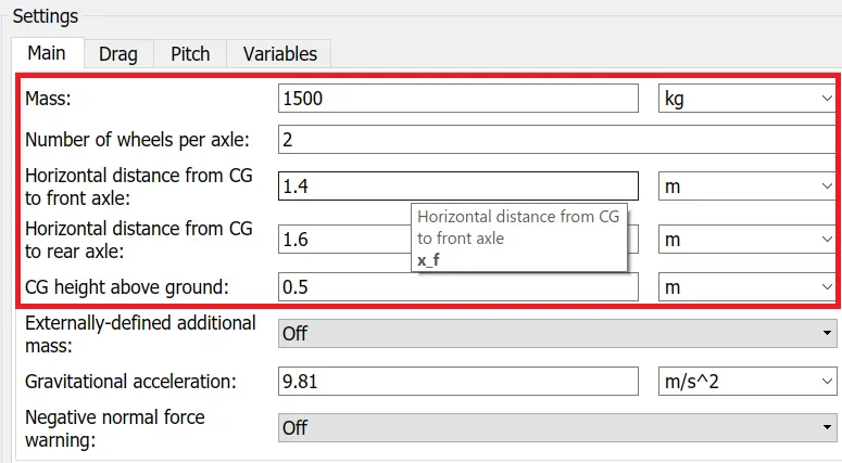
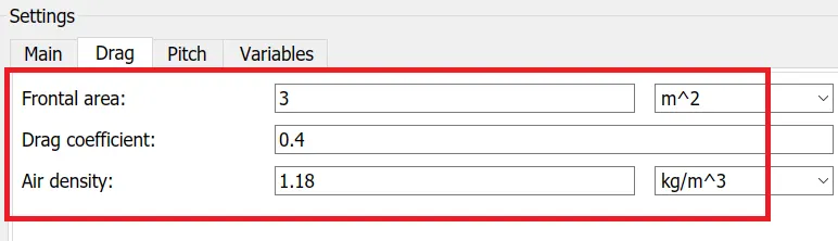
This block represents a two-axis body moving longitudinally. This unit takes into account body weight, air resistance, road slope and weight distribution between axles due to acceleration and road profile. This unit allows for the same or different number of wheels on each axle and can optionally include pitch and suspension dynamics or additional variable mass and inertia. The mass of the body does not move vertically relative to the ground.
The block consists of a total of 6 connection ports; where "H" is the mechanical transient protection port associated with the horizontal movement of the body which is connected to the "H" port on the tire hub through which the tire thrust movement will be generated. "V" is a physical output port used to control and monitor the vehicle's speed curve, "NF" and "NR" are also physical output ports, but they represent the normal forces of the front and rear wheels, so they are connected to "N" the tire through the force acting on it. When turning the steering wheel, “W” and “beta” are physical signal input ports corresponding to headwind speed and road gradient.
The parameter values assigned to the body are as follows:
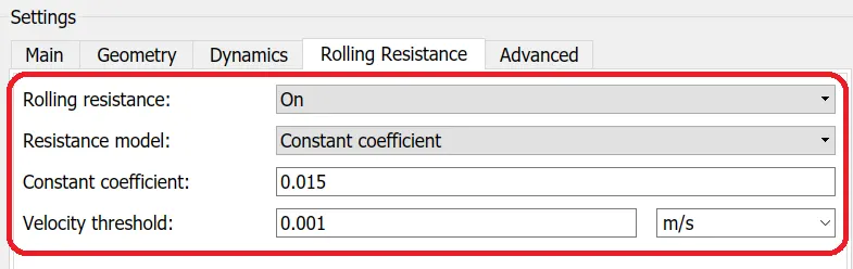
ii) Tire(Magic Formula):

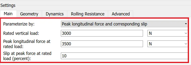
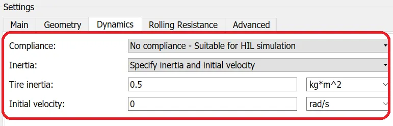
The tire block (Magic Formula) models a tire with longitudinal behavior defined by the magic formula [1], which is an empirical equation based on four fitted coefficients. This module can simulate tire dynamics under constant or changing road conditions. The longitudinal direction of the tire is the same as the direction of movement when it rolls on the road. Attributes such as tire compliance, inertia and rolling resistance can be specified to improve the reliability of the tire model. However, these properties increase the complexity of the tire model and slow down the simulation. If you are modeling the model in real-time or preparing the model for hardware-in-the-loop (HIL) simulation, consider ignoring tire compliance and inertia.
Like the body, the block also consists of 4 connection ports; where 'A' is the mechanical pivot point of the axle that engages the vehicle gear. The "H" is a mechanical displacement saving port on the hub through which the vehicle tires pressurize, it is connected to the "H" port on the housing to initiate horizontal movement. “N” is a physical signal input port for the normal force applied to the tire which is connected to “NR” and “NF” on the body.
The parameter values assigned to decks are as follows:

iii) Simple Gear:

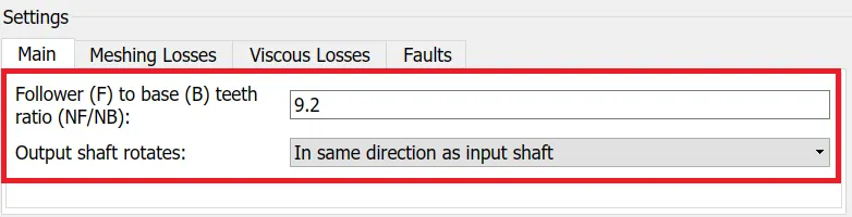
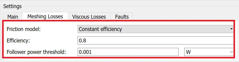
This block represents a fixed gear or gearbox. This block does not model inertia or compliance. You can choose to include gear engagement and viscous bearing losses.
Connections B (base) and F (follower) are mechanically shielded ports that connect to the DC motor shaft input and the "A" port on the wheel shaft. The relationship between the direction of rotation of the base and the follower and the rotation parameter of the output shaft.
The parameter selection values for a simple gear are as follows:
iv) Inertia:

This block represents the ideal mechanical moment of inertia. The positive direction of the block is from its gate to the reference point, which means that if inertia accelerates in a positive direction, the moment of inertia is positive. The inertia value is chosen to be 4kg*m2.
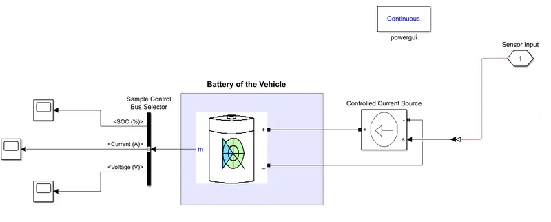
Battery Management Subsystem:
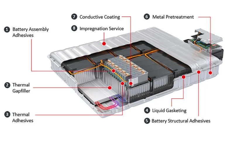
The BMS will also manage battery charging by channeling recovered energy (ie from regenerative braking) back to the battery pack (typically made up of multiple battery modules, each composed of multiple cells). Battery thermal management systems can be passive or active, and the cooling medium can be air, liquid, or some form of phase change. The advantage of air cooling is its simplicity. Such systems can be passive, relying only on ambient air convection, or active, using fans to provide airflow. Commercially, both the Honda Insight and Toyota Prius use active air to cool their battery systems.
The main disadvantage of air cooling is its inefficiency. It takes a lot of power to run the cooling mechanism, much more than active liquid cooling. Additional components for the cooling mechanism also increase the weight of the BMS, reducing the efficiency of the battery for transportation. Liquid cooling has a greater free cooling potential than air cooling because liquid refrigerants have a higher thermal conductivity than air. The battery can be immersed directly in the coolant, or the coolant can flow through the BMS without directly touching the battery. Indirect cooling has the potential to create large thermal gradients across the BMS due to the increased length of the cooling channels. This can be reduced by pumping the coolant through the system faster, creating a trade-off between pumping speed and thermal consistency.
The subsystem configuration is as follows:
i) Battery:
This module implements a general dynamic model representing the most popular types of rechargeable batteries if:
It is assumed that the internal resistance remains constant during charge and discharge cycles and does not change with the magnitude of the current.
The model parameters are derived from the discharge characteristics. The discharge and charge characteristics are assumed to be the same.
Battery capacity does not change with current (no Perquet effect). Battery self-discharge is not displayed. This can be represented by placing a large resistor in parallel across the battery terminals.
The equivalent circuit of the battery pack is shown in the figure below:
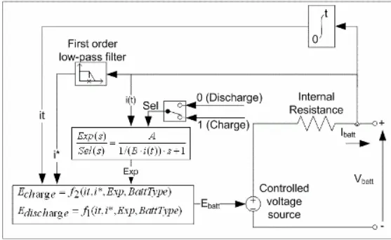
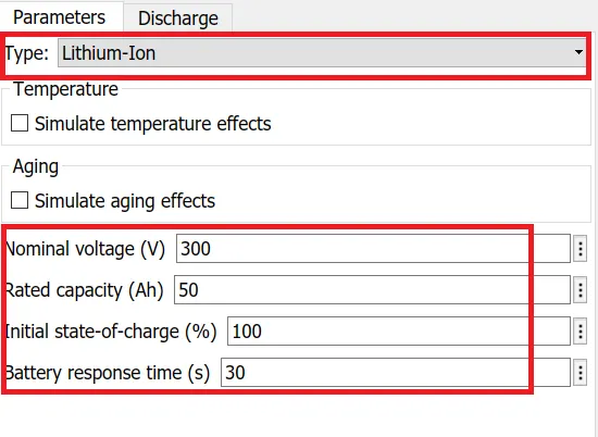
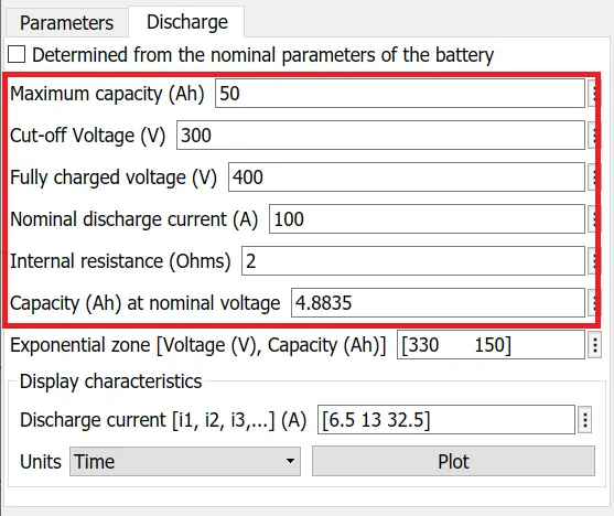
As the battery charges, the voltage drops exponentially depending on the type of battery. Because the battery is rechargeable, a significant amount of charge can be drawn from the battery until the voltage drops below the rated voltage of the battery. According to the project requirements, the nominal voltage of the battery is set to 300 V and the initial SOC is 100%.
The positive terminal of the battery is connected to a controlled current source unit where the current is controlled based on the voltage of the DC motor.
The battery set parameter values are shown in the figure below:
ii) Controlled Current Source:

This block is responsible for converting the Simulink input signal into an equivalent current source. The generated current is driven by the input signal of the block. The block is initialized as an AC source type and the simulation starts at steady state conditions, so the input of the block must be connected to a signal that starts with a sine or DC waveform corresponding to the initial value.
The positive and negative terminals of the module are connected across the battery and the physical port "S" is connected to the physical output port "I" of the current sensor of the DC motor subsystem. It is arranged so that the current drawn by the DC motor comes from the common battery.
SOC Estimation Subsystem:
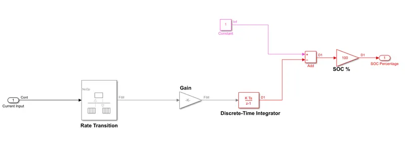
i) Rate Transition:

A speed transition block transfers data from the output of a block operating at one speed to the input of a block operating at another speed. Use the block parameter to offset data integrity and deterministic transfers for faster response or lower memory requirements. The operation of the speed transfer unit depends on the following conditions:
- The sample time of the port the block is connected to.
- Task priority for source and destination sample times. Does the model specify a fixed or variable step solver.
- Model configuration parameter settings.
As required by the design, the output state is held at zero and the sampling time of the output port is specified with an amplitude of -1.
ii) Discrete Time Integrator:

This module is used to create pure discrete models. This block helps define the following scenarios:
- Start conditions in a block dialog box or as block input
- Enter the gain (K) value
- output block status
- Integrated upper and lower bounds
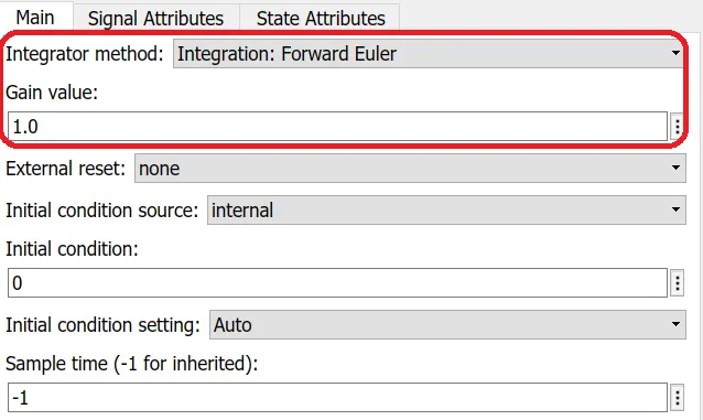
According to the Inetgrator project, the method is chosen as the direct Euler method, the gain value is 1.0, there is no initial condition, and the sampling time is -1.
The parameters of such selected blocks are as follows:
iii) Gain:

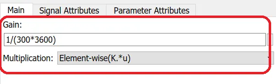
The gain block multiplies the input by a constant value (gain) Both the input and the gain can be scalars, vectors, or matrices. The gain values are specified in the gain parameters section of the block. The multiply parameter allows the user to specify the multiplication of an element or matrix. For matrix multiplication, this parameter also allows you to specify the order of the multipliers. The gain value is shown in the figure below:
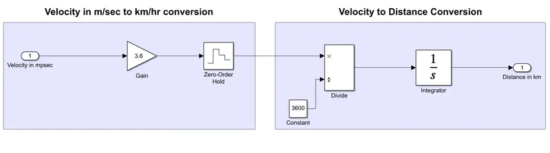
Distance calculation subsystem:
The subsystem configuration is shown in the figure below:
 i) Zero order command:

This block is used to store the input amplitude for a user specified sampling period. If the input is a vector, the block will store all elements of the vector with the same sampling period. The user must specify the test time parameter, which is set to -1 by default. A zero-order hold block is a bus-enabled block. Inputs can be virtual or non-virtual bus signals. There are no block-specific restrictions. All signals on the non-virtual bus inputs of the zero-order latch block must have the same sample time, even if the elements in the associated bus object specify a legacy sample time.
ii) Integrators:

This block produces an output that is the integral of its input signal with respect to time. The selected solver calculates the output of the integrator block at the current time step using the current input values and the state values from the previous time step. To support this calculation model, the integrator block stores its output at the current time step, which is used by the solver to calculate the output at the next time step. The block also provides the initial conditions for the solver, which is used to calculate the initial state of the block at the beginning of the simulation. The initial condition defaults to 0. Use the Block Parameters dialog box to specify a different initial condition value or to create initial values in the input port block.
Energy calculation subsystem:
The subsystem configuration is as follows:
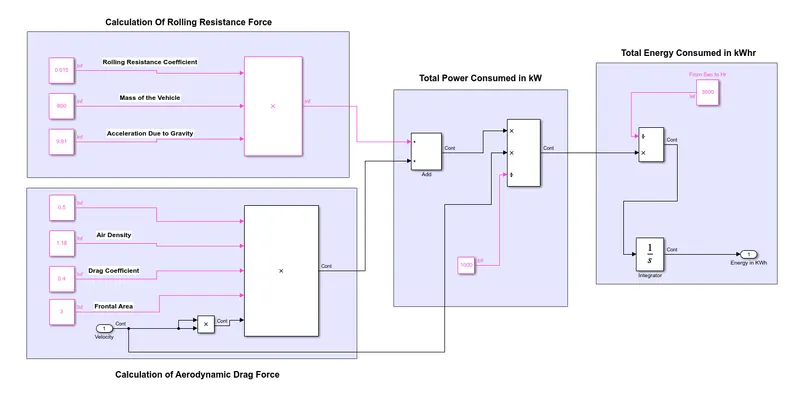
In this design, the vehicle is assumed to be traveling on level ground, so the slope is assumed to be zero, which ultimately makes the climbing force equal to zero.
After calculating the force, the corresponding power is calculated by multiplying the force by the corresponding vehicle speed point as the output of the vehicle dynamic subsystem. Combining this effect with time will yield the vehicle's final energy consumption for a given driving cycle source.
Considering the size of the vehicle battery, the energy calculation is very important. Knowing the vehicle's average energy consumption and range can optimize the battery's dynamic performance and charging time.
Results and discussion:
According to the project requirements, the performance characteristics of the EV model were analyzed for three different driving cycle sources; the three driving cycles were FTP75, WOT and an adapted driving cycle following a constant speed of 45 km/h which is 12 mpsec for a total of 100 km. Check all the performance parameters like vehicle speed, SOC, voltage and current consumed by the motor etc. according to each cycle and create a profile in the next section.
Case 1: Loop source is FTP75:
FTP-75 (Federal Test Procedure) is used in the United States for light vehicle emissions certification and fuel economy testing. This test is often referred to simply as "FTP" (not to be confused with the FTP test for heavy duty engines). The "city" driving program in the EPA federal test procedure is the same as the UDDS plus the first 505 seconds of the additional UDDS loop.
The speed profile of this driving cycle has the following characteristics:
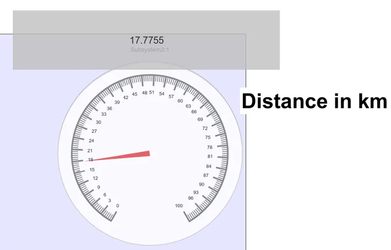
- Driving distance: 17.77 km (11.04 miles)
- Duration: 1874 seconds
- Average speed: 34.1 km/h (21.2 mph)
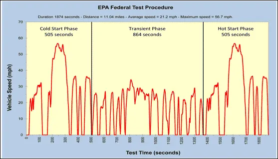
A typical FTP75 drive cycle.
Before comparing the actual speed to the reference speed, it is important to understand the role of the PID controller in the response of the machine, so compare after tuning and after tuning and after tuning the PID controller to understand its effect on the system output. The role of response.
Before tuning:
For this drive cycle source, the corresponding vehicle speed compared to the drive cycle reference speed is:
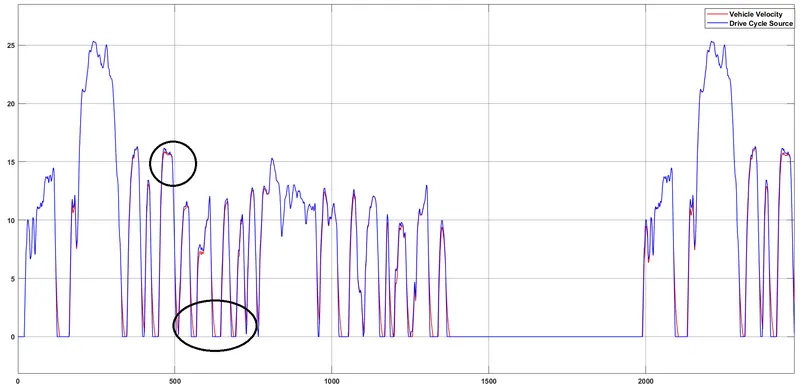
By zooming the results, we can see that 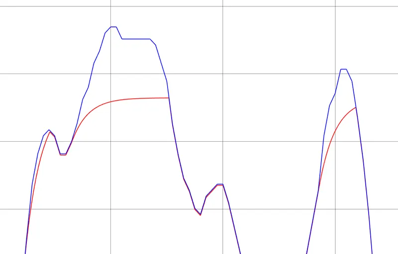 Upper part of the curve (peak)
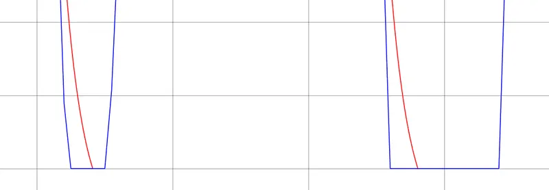
lower part of the curve.
From the above two cases, we can see that if the PID controller is not set correctly, the speed response can vary greatly, which can become a dangerous situation in real-time situations, even with a small fraction of the actual speed deviation from the reference. Riding a bicycle at a speed that may cause unexpected or dangerous situations. Therefore, to prevent this problem, the PID controller must be perfectly tuned.
After tuning:
These errors are greatly reduced by using a properly tuned PID controller as follows:
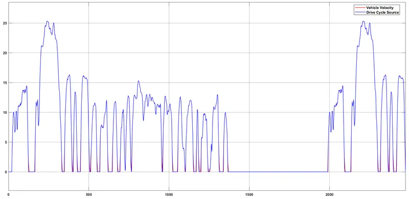
Therefore, it can be seen from the above figure that the speed output error is greatly reduced.
Below are the corresponding temperature profiles for the vehicle's PMDC engine and its converter:
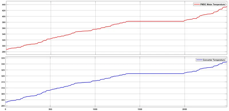
From the picture we can clearly see; from the moment the vehicle starts to respect the reference speed, the temperature of the engine and its converter starts to rise linearly, while the engine and its converter continue to operate to provide torque to continuously generate the vehicle speed for about 1400 seconds, after which the reference speed becomes zero, therefore the temperature of the motor and inverter remains constant up to 2000 seconds, after which the temperature starts to rise again due to the change in the reference speed curve.
The SOC evaluation curve is as follows:
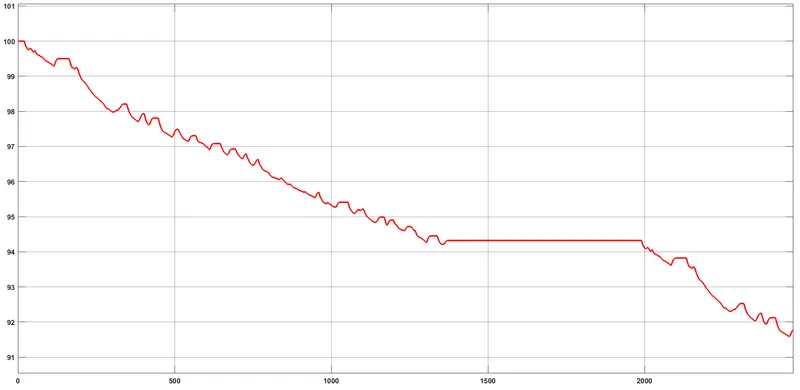
From the graph it can be seen that as the vehicle increases, the battery charge level decreases, the peak of the curve occurs due to regenerative braking conditions, in this case the battery is charged due to the opposite current flow due to the deceleration of the vehicle. As can be seen from the curve, after completing the cycle, the remaining charge of the battery is 91.81%, so the battery drains about 9% of its charge to complete the above cycle.
The nature of the current consumed by the motor is as follows:
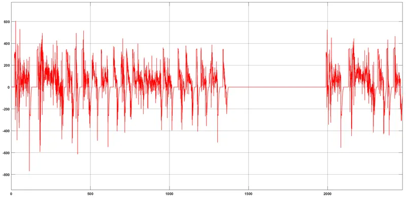
PMDC motor current curve
The above two curves can show that as the vehicle accelerates, the current increases from its initial value as the threshold of the motor increases. However, when the vehicle decelerates, the regenerative braking condition of the motor is satisfied, so since the direction of rotation of the motor is reversed, the current moves to the negative axis, which clearly proves the regenerative phenomenon of the motor when the vehicle decelerates.
The distance profile of the vehicle is shown in the figure below:
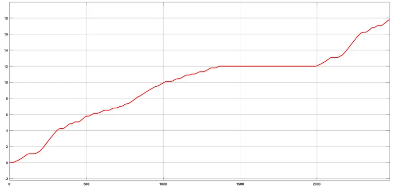
This is a curve of the distance traveled by the vehicle at the reference speed of the driving cycle. The total distance (in kilometers) traveled by the vehicle after the end of the loop is also measured using the MATLAB "display block" as follows:
The car's energy consumption profile is shown below:
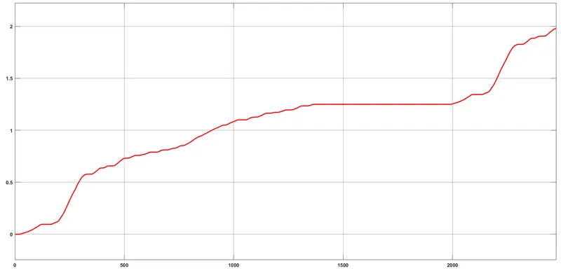
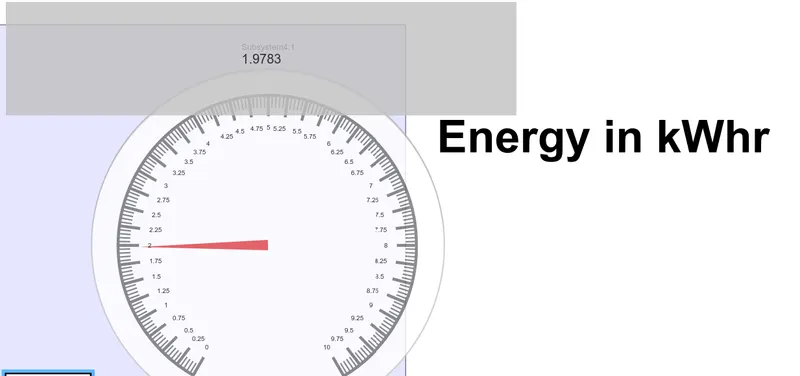
This is the energy consumption profile covered by the vehicle at the source reference speed of the driving cycle. The total energy (kWh) consumed by the vehicle at the end of the cycle is also measured using the MATLAB display block as follows:
Case 2: Drive loop source is WOT:
under wide open throttle (WOT) conditions; due to the high engine torque production associated with WOT conditions and no load added to the engine, the engine speed suddenly increases. The engine's acoustic emissions contain information related to this increase in speed and thus the engine's torque generation. The method reveals information in the acoustic emissions of the engine to estimate the torque produced under WOT operating conditions. This evaluation can be done without connecting the engine to the brakes and without installing additional sensors.
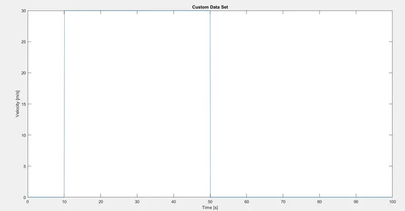
WOT driving cycle.
For this drive cycle source, the corresponding vehicle speed compared to the drive cycle reference speed is:
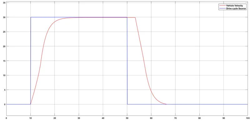
As shown in the figure above, due to the limitations of the vehicle's internal circuit, it is not possible to achieve a rapid increase in the reference speed, so it increases linearly from 10 seconds and another 15 seconds to reach full speed. ideal speed value. Even during deceleration, the vehicle speed increases to approx. 15 seconds to return from maximum to zero position due to vehicle inertia.
The corresponding temperature profiles for the vehicle's PMDC engine and its converter are shown below:
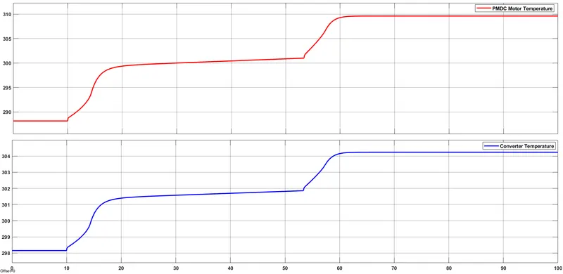
From the nature of the curves, we can clearly understand that during acceleration of the vehicle, the corresponding engine and converter temperatures rise from 298.15 degrees K to approx. Motor torque increase of 301 degrees K (inverter) and from 288.05 degrees K to 299 degrees K (motor). Even when operating at a constant maximum speed, the temperature of the motor and its converter rises slightly by about 0.4°K, which is mainly due to the continuous operation of the motor and converter. In addition, during the deceleration of the vehicle, due to the phenomenon of regenerative braking, the temperature of the engine and its control unit will rise rapidly and finally stabilize at the maximum temperature. During the whole cycle, the converter temperature rise is 10-11°K, and the engine temperature rise is 20-22°K, respectively.
The SOC evaluation curve is as follows:
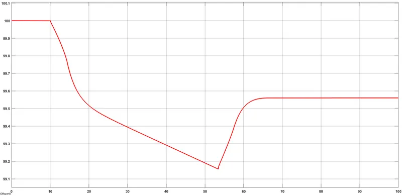
As can be seen from the above curve, during the acceleration of the vehicle, the general battery discharges from 100% to 99.18% in 53 seconds, i.e. the time from acceleration of the vehicle to cruising at a constant top speed is about 50 seconds at most, so during deceleration the engine will reverse due to regenerative braking, thus current will flow into the battery, so it regains some charge and eventually settles at 99.54%. Since the duration of the WOT driving cycle is shorter compared to other driving cycles, very little current is drawn.
Current drawn by motor is as shown below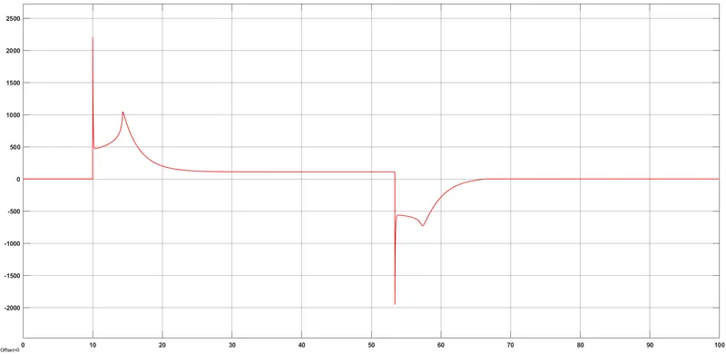
Permanent magnet DC motor.
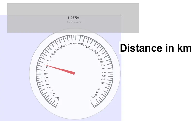
The above two curves correspond to the voltage and current of the PMDC motor, which is exactly the same in nature as the previous FTP75 drive cycle. The distance profile of the vehicle is shown in the figure below:
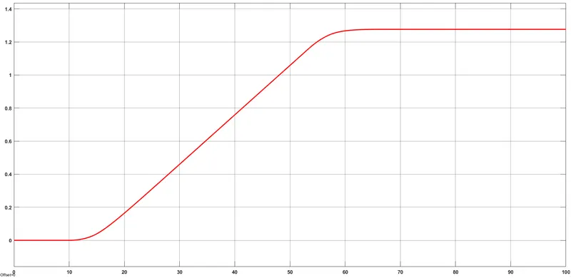
This is a curve of the distance traveled by the vehicle at the reference speed of the driving cycle. The total distance (in kilometers) traveled by the vehicle after the end of the loop is also measured using the MATLAB "display block" as follows:
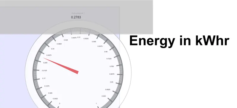
The car's energy consumption profile is shown below:
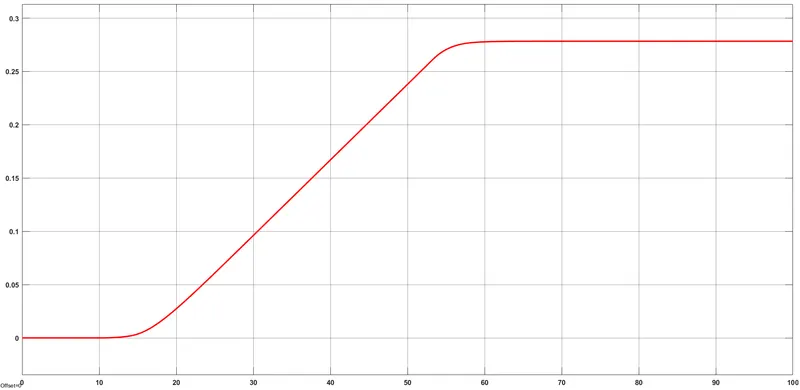
This is the energy consumption profile covered by the vehicle at the source reference speed of the driving cycle. The total energy (kWh) consumed by the vehicle at the end of the cycle is also measured using the MATLAB display block as follows:
Case 3: 45 km/h constant speed 100 km adapted driving cycle:
Here give the system a constant 45km/h i.e. 12.5msec as a reference for 8000sec. to reach a distance of 100 km.
For this drive cycle source, the corresponding vehicle speed compared to the drive cycle reference speed is:
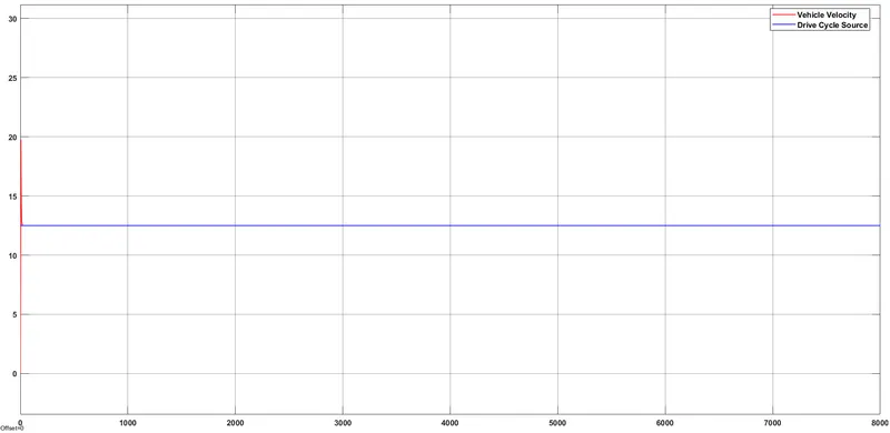
Here, after an initial increase due to a sudden jump in vehicle speed from 0 to 12.5 msec, the vehicle speed maintains a constant speed profile according to the reference speed.
The corresponding temperature profiles for the vehicle's PMDC engine and its converter are shown below:
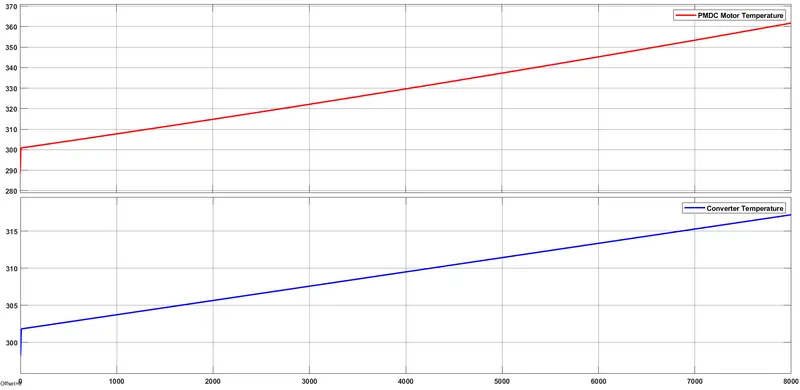
Since the speed is kept constant at 12.5mps for 8000 seconds to cover a total distance of 100km, the temperature of the motor and its converter will also increase linearly above 370°K for the motor and 317°K for its converter.
The SOC evaluation curve is as follows:
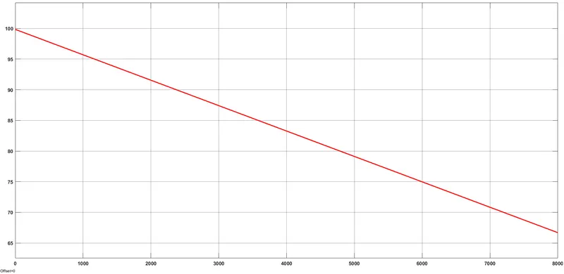
Here, the SOC of the battery will decrease linearly to 66%, which is about 34% of the discharged battery. The nature of the current consumed by the motor is as follows:
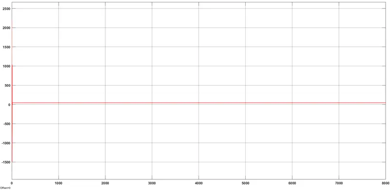
Current curve for PMDC motor.
It is clear from these two graphs that since there is no regenerative braking, the motor current and voltage are constant throughout the cycle and are on the positive axis.
The distance profile of the vehicle is shown in the figure below:
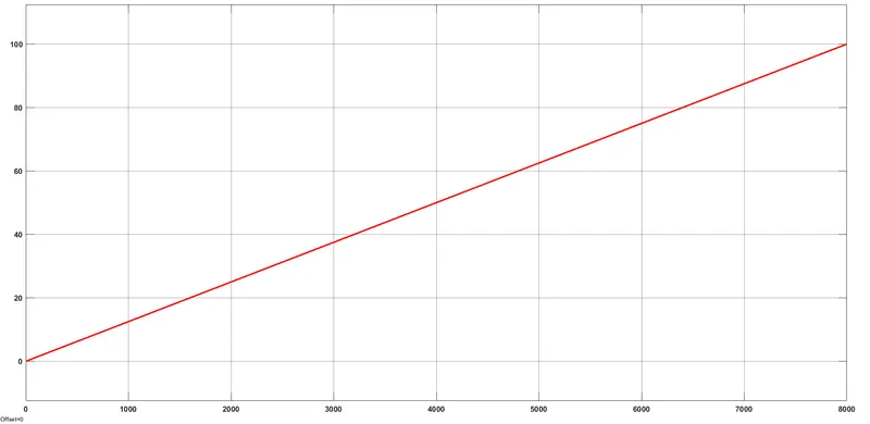
This is a curve of the distance traveled by the vehicle at the reference speed of the driving cycle. The total distance (in kilometers) traveled by the vehicle after the end of the loop is also measured using the MATLAB "display block" as follows: Here the distance increases linearly to 100 km.
The car's energy consumption profile is shown below:
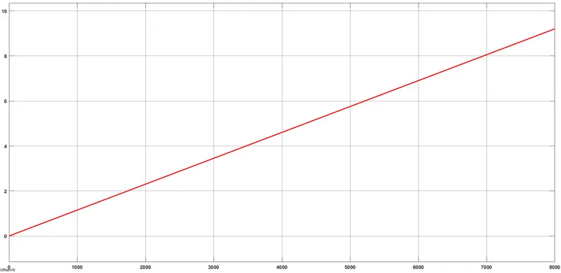
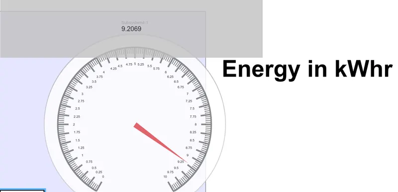
This is the energy consumption profile covered by the vehicle at the source reference speed of the driving cycle. The total energy (kWh) consumed by the vehicle at the end of the cycle is also measured using the MATLAB display block as follows:
Conclusion:
Therefore, the performance characteristics of the MATLAB electric vehicle model were successfully obtained by obtaining various driving cycle sources and carefully studying the results through detailed analysis and discussion. All the required results for each driving cycle are displayed together with a detailed description of the model pieces with parameters.