Project 1 - Data Cleaning and Transformation using Pivot table and Charts for the Report on requirement of Team Hiring

Project 1

a. Do proper formatting of the data with using borders, font size and appropriate alignment of the content.

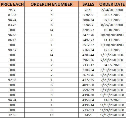
• Used a bold heading for the columns and filled it with different color
• Used Calibri -14 for the columns heading
• And used Calibri -14 for the datas.

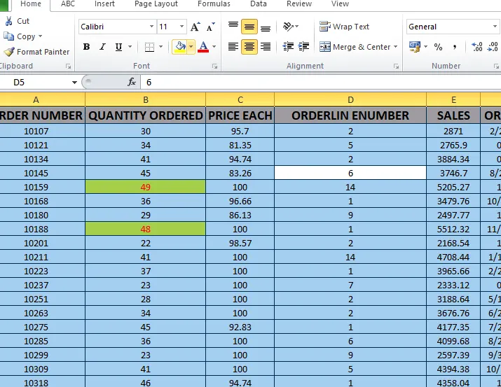
• Alligned at the center
• Created the All borders
• Shown in formatted data worksheet

b. Make summary of Products Sales by providing

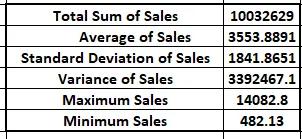
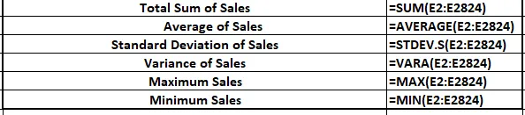
• By using the formulas obtained sum , average , std dev , variance, min and max of sales.
• Show in formatted data worksheet.

c. Analyse the sales happened by product line & status using pivot table

• Selected the entire dataset and from insert tab used pivot option

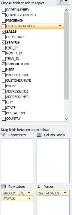
• Selected Productline and status under Row Labels
• Sum of Sales under volume selected the sum

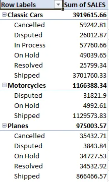
• Shown in worksheet called Pivot table.

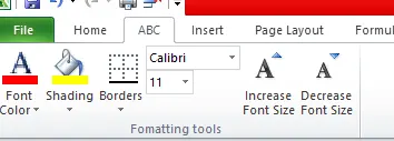
d. Make Customized Tab by naming ABC and keep few data formatting commands in the newly created Tab.

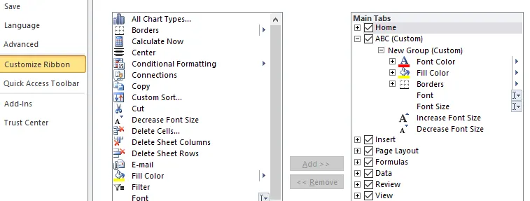
• Rigt clicked on tool bar and the selected customize Ribbon

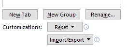
• Selected the new form the option named it as ABC
• Created the new group called Formatting tools.
• Added tools to increase and reduce the Font size , fill color option and also borders option
• Shown in formatted data worksheet.

e. Analyse the Quantities ordered by each Country in Year 2019,2020 and 2021 for different Quarters using Pivot Table.

• Selected the entire dataset and from insert tab used pivot option.

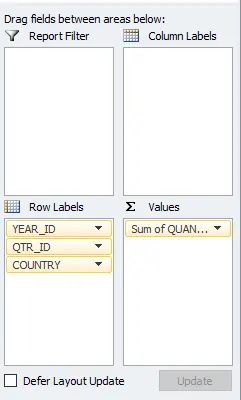
• Added the year_id, QTR _id and country colums to the Row labels
• Quantity orderd under the values and got the sum of quantities.

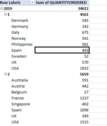
• Show in pivot worksheet

f. Present the data in different colours for values in field Status and ProductLine using conditional formatting.

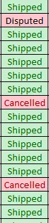
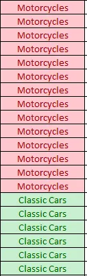
• Used different colors for different status like for cancelled it is filled with light red with font red color etc.
• Used different colors for different product line like Motorcycles used red filled with light red with font red color and for Classic Cars filled with light green with font color as dark green.
• Show in formatted Data worksheet.

g. change values of 2003 to 2019, 2004 to 2020 and 2005 to 2021 by using proper date formatting options.

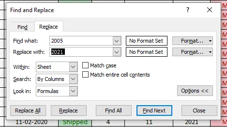
• I utilized the "Ctrl + F" shortcut to initiate the Find and Replace function, navigating to the replace tab. Within the "Find what" field, I entered "2005" as the search term, and in the "Replace with" field, I specified "2021" as the replacement value, followed same process for rest of the values.
• Show in formatted Data worksheet

h. Calculate the total sales of all “Shipped”, “Cancelled”, “Disputed”, “In Process”, “On Hold”, “Resolved” products. (Hint:Use pivot table or sumif function)

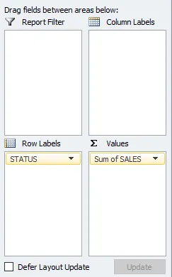
• Used the pivot table to get sum of sales of each status.
• Used status column under the row labels
• Used Sum of sales under the values.

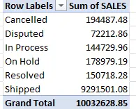
• Show in pivot worksheet

i. Split the productcode field into two using text functions Example :S10_1678 -> S10 in one column and 1678 in another column.

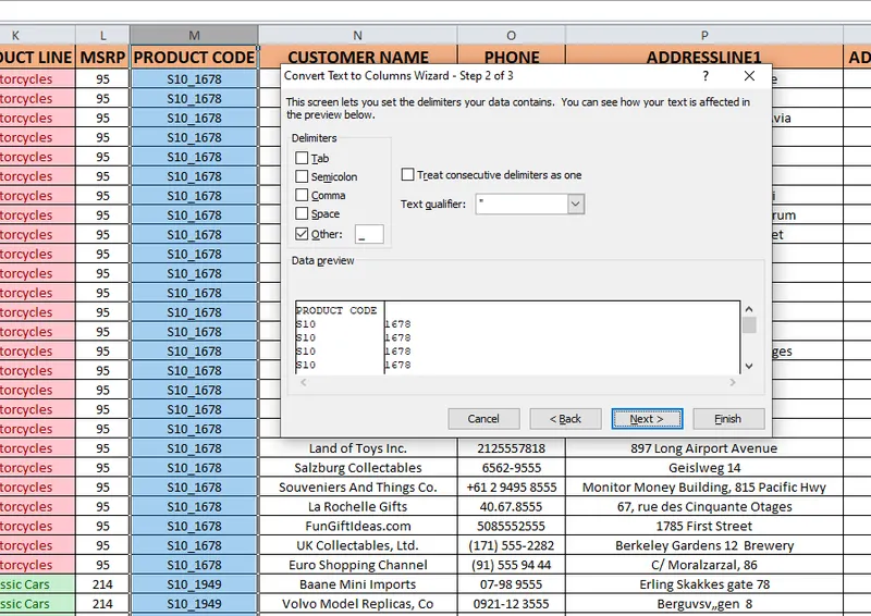
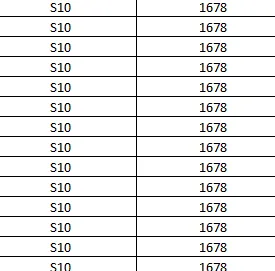
• From the data tab used "test to column" option and used to delimiter as "_" choose the destination cell
• Got the values in two different columns
• Shown in Formatted data worksheet

j. Highlight the top 10% values of QuantityOrdered field using Conditional Formatting

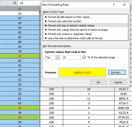
• Selected entire column used conditional formatting option form home tab
• called format only top or bottom ranked value
• Used Top 10 values checked % option.
• Show in formatted Data worksheet

Attached the excel file below which has 3 worksheets , pivot table , Formatted data type and original data