Project 1
PROJECT 1: Development of a Forward energy-based Fuel Consumption Model of a Conventional Vehicle
Aim:
The aim of this project is to compute the fuel economy numbers for the given vehicle (km/L) on the UDDS and HWFET Cycle. Also, to analyze and understand the vehicle operating points in terms of engine speed, torque, power, transmission speeds, pedal positions, gear, distance traveled, etc.
Tasks:
- Build the engine and vehicle dynamics blocks for the given vehicle model.
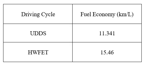
- Tabulate the fuel economy numbers (km/L) for UDDS and HWFET cycle.
- Plot the time trace for engine, transmission input, transmission output and wheel speed on one plot.
- Plot engine torque, engine power, fuel rate and fuel consumption using subplots.
- Plot accelerator and brake pedal, gear command, vehicle desired and actual speed, vehicle distance using subplots.
- Plot the engine operating points on the engine fuel map.
Plots must be created for both the cycles.
Theory:
Forward model of a vehicle:
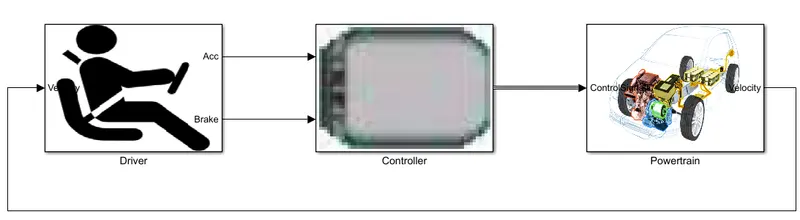
In a forward model, information flow takes place between Powertrain block and Driver block as well as between Driver block and Controller block. The driver receives the information through the odometer and the consoles present. Based on this information, the driver takes an action which is then passed onto the powertrain through a controller. The controller receives the information from the driver, where it translates the information and makes necessary changes and applies it onto the powertrain, which brings the changes made by the controller into action. This therefore represents a feedback loop. The controller acts as an interface between driver and powertrain, which allows the communication between both the components.
Driver Model:
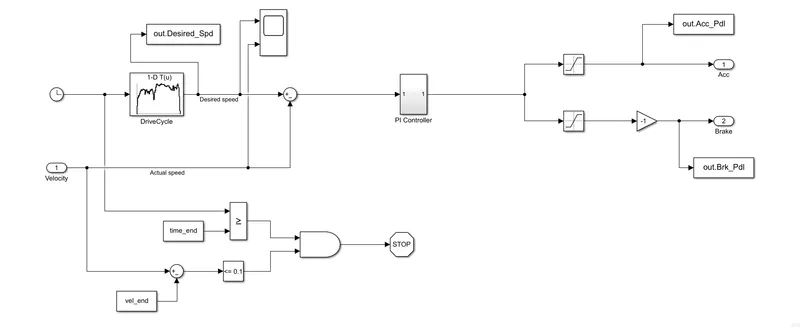
The driver block mainly contains a PI-Controller, which helps to maintain the vehicle speed at the desired speed. Here the desired speed is obtained from the driving cycle and the actual speed is taken from the Powertrain block. The input for the controller is the difference between the desired and actual speed or so to say the error in speed. The error then passes through the proportional and integral paths, both with defined gains, and gets added up. The controller output is then divided into two, where positive values represent the need to accelerate and negative values represent braking. These values are also transferred back into the MATLAB Workspace. The outputs of the driver block are therefore the accelerator or throttle pedal position and the brake pedal position in percentage (the saturation blocks converts the error values into the limits 0-100), which then go into the Controller block as its inputs.
Controller Block:
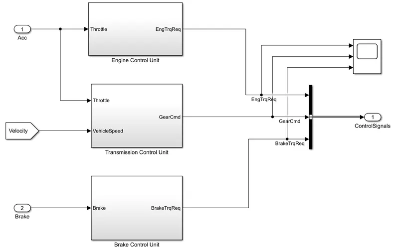
The controller block is the brain of the vehicle. It contains an Engine Control unit (ECU), Transmission Control and Brake Control Units. The ECU converts the throttle request from the driver into torque request for the powertrain, specifically the engine. It also contains an idle speed controller that defines the idle throttle position based on the engine speed. The transmission control unit outputs the gear that is to be used based on the throttle position and vehicle speed. The shifting logic of the gears is modelled in StateFlow. The brake control unit basically converts the brake pedal position into a brake torque request.
The major purpose of the controller block is to create the torque requests and gear choices based on the driver input. It acts as the link between vehicle and driver, as it translates the drivers requirements into powertrain requirements. The outputs of the block are sent to the powertrain through bus. The bus interconnects different components inside a vehicle.
Powertrain Block:
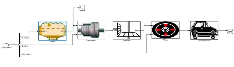
The powertrain block is the block representation of the actual powertrain of a vehicle. It receives the input from the controller and produces the outputs based on it. The torque request from the controller goes into the engine, where the engine produces the necessary torque based on the request. The engine is connected to the transmission through a torque converter. The transmission block receives the desired gear choice from the controller. The engine torque gets converted into the transmission input torque (torque converter does the conversion), which gets multiplied with the gear ratio of the desired gear and thereby forms the transmission output torque. The transmission is connected to the differential, which converts the rotation of the drive shaft to the rotation of wheels. The purpose of the differential is to allow the inner and outer wheels of the vehicle during a turn to rotate properly; the outer wheel rotates faster than the inner as it travels more distance in a turn. The differential is a kind of gear and it has gear ratio, which get multiplied with the torque value. The differential drives the wheels, which provides traction to the vehicle. The wheel receives the torque from the engine and also the brake torque request generated by the controller. The difference of the both along with the rolling radius of the wheel forms the tractive force. The tractive force then needs to compared with the resistance forces (or road load) developed due to the vehicle, to obtain the net force which drives the vehicle forward. This is basically modelled in the Vehicle Dynamics block. It basically contains the physical relations that define dynamics of the vehicle, where actual physical components like the rolling resistance, drag resistance and the resistance due to gradience are calculated, which forms the road load and are subtracted from the available tractive force to obtain the net force. For the vehicle to move forward, the tractive force must always be greater than the road load. From the net force, the acceleration, the velocity and the distance covered by the vehicle are calculated.
The velocity obtained from the powertrain block represents the actual velocity of the vehicle. This value then goes into the driver block, where it is compared against the desired velocity. For this project the vehicle needs to traverse the given driving cycles (UDDS and HWFET), therefore the desired velocity values are obtained from the driving cycle. Errors in the values gets controlled by the PI-Controller, which therefore generates the throttle and brake positions that are required to minimize the error. These values then go into the Controller block and the whole process repeats, until there is no error or until the desired condition is reached.
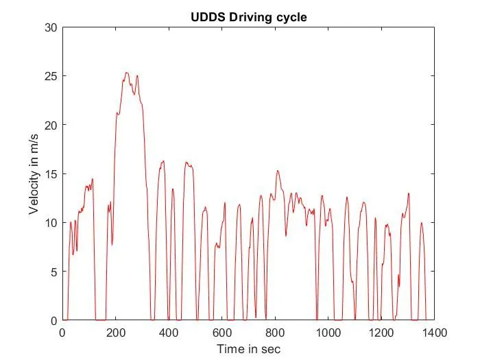
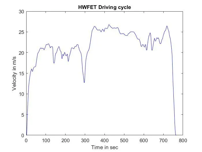
For this project, a typical midsize car with a 1.9L engine and a 4-speed automatic transmission (Saturn 1.9L) is considered. Data is taken from ADVISOR data base developed by NREL, USA. Transmission shift map and controller is taken from Matlab/Simulink example database. The driving cycle data for UDDS and HWFET cycles are also given.
Urban Dynamometer Driving Schedule (UDDS):
Highway Fuel Economy Test (HWFET):
Mathematical Relations:
- Angular speed, `omega = 2*pi*(N/60)` , where N is the speed in rpm
- Power, `P = tau*omega` , where `tau` is the torque in Nm
- Fuel economy, `kmpl = D/F * rho_F,`, where D is the distance covered in km, F is the fuel consumption in kg and `rho_F`is the density of the fuel in kg/L. F and D are time dependent parameters.
MATLAB/Simulink Data:
Two MATLAB Scripts and a Simulink model of the vehicle are provided. In the MATLAB Scripts, one contains all the variables necessary to run the Simulink model and the other one is used to process the data generated from simulating the model, which basically involves some mathematical calculations and also generating the necessary plots as per the aim of the project.
Methodology:
Initialization:
In order to create a model in Simulink, variables are required. All the necessary variable must be initialized in the MATLAB Workspace, so that they can be used while modelling. Therefore to initialize all the variable a MATLAB Script is created. The script also loads the engine data and transmission data from external files, along with which, the drive cycle selection is also done (user defined). Executing the script initializes all the necessary parameters in the workspace.
MATLAB Script:
%%%%%%%%%%%%%%%%%%%%%%%%%%%%%%%%%%%%%%%%%%%%%%%%%%%%%%%%%%%%%%%%%%%%%
%% Skill-Lync -> Hybrid Drives Development
% Project 1 - Conventional Vehicle Model

%% Initialization File
% Initialization file for loading the variables for the Conventional vehicle simulation model

%% Vehicle Parameters
M = 1500;           % Vehicle weight [kg]
Cr = 0.015;         % Rolling resistance coefficient
Rw = 0.35;          % Rolling radius [m]
Cd = 0.33;          % Drag coefficient
Af = 2;             % Frontal area [m2]
rhoa = 1.225;       % Air density [kg/m3]
Vwind = 0;          % Wind velocity [kmph]
g = 9.81;           % Gravitational acceleration [m/s2]
theta = 0;          % Slope [deg]
myu_road_tire = 1;  % Coefficient of friction between tire - road interface

%% Powertrain Parameters
FDR = 3.73;                         % Final Drive Ratio / Diff Ratio
DiffEff = 0.99;                     % Differential efficiency (assumed independent of operating conditions)

NumGear = 4;                        % Number of gears in transmission
TransGear = [1:NumGear];            % Transmission Gears
TransRatio = [3.06, 1.62, 1, 0.7];  % Corresponding Transmission ratios
TransEff = 0.90;                    % Transmission efficiency (assumed independent of operating conditions)

TC_SR = [0, .5, .6, .7, .8, .87, .92, .94, .96, .97, 1];   % Torque Converter Speed Ratio (Matlab default) -> TurbSpd/PumpSpd
TC_TR = [2.232, 1.5462, 1.4058, 1.2746, 1.1528, 1.0732, 1.0192, 1, 1, 1, 1];   % Torque Converter Torque Ratio (Matlab default) -> TurbTrq/PumpTrq
TC_Cf = 1e-4 * [.72558, .66322, .63463, .59042, .51331, .4144, .29287, .22444, .12186, .04386, 0]; % Torque Converter Capacity Factor (Matlab default) -> PumpTrq/PumpSpd^2 [Nm/rpm^2]

load Vehicle_Data/Engine_data_1_9L_Saturn_95kW
load Vehicle_Data/Trans_Shift_map

%% Driver Parameters
Kp = 10;                    % P gain for driver PI model
Ki = 1;                     % I gain for driver PI model
Drive_Cycle_Select = 1;     % Drive cycle selection

% Drive cycle values in m/s

if Drive_Cycle_Select == 1
    load DriveCycles/UDDS;

elseif Drive_Cycle_Select == 2
    load DriveCycles/HWFET;

end

time_end = cyc_time(end);
vel_end = cyc_vel(end);
Modelling in Simulink:
Once the variables are initialized, the forward model of the vehicle can be modelled in Simulink. For this project a model of the vehicle is given with certain missing components. These components - engine and vehicle dynamics block - therefore needs to be developed.
Engine Block:
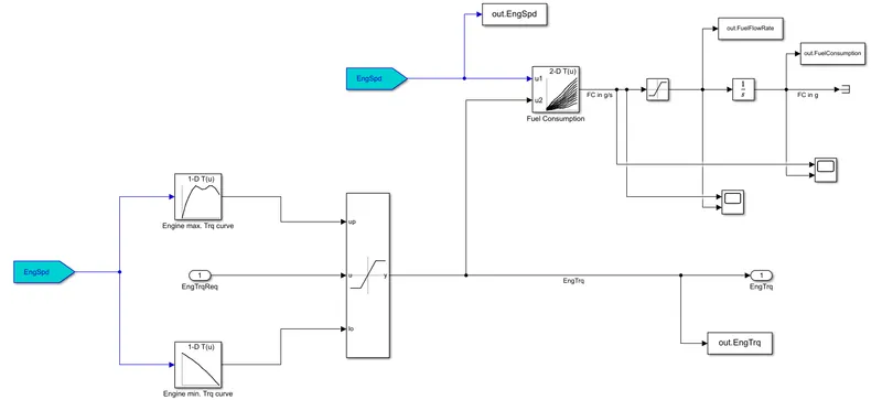
The engine block has mainly two inputs - the torque request from the controller and the engine speed. The torque request is generated by the controller based on the driver input, basically the throttle position determines the torque request. The engine speed is obtained from the torque converter in the transmission block. The outputs from the engine block is mainly the engine torque, the torque produced by the engine as per the request from the controller.
Using the engine speed, the maximum and minimum torque that can be produced by the engine at that speed are obtained. The maximum and minimum torque curves of the engine are initialized using the intialization script based on the available engine data. The torque request generated by the controller is bound between the maximum and minimum torque values of the engine using a dynamic saturation block in Simulink. It basically sets an upper and lower limit for the torque request. This therefore creates the torque that needs to be generated by the engine.
The fuel consumption of the engine is also determined from this block. After engine torque is determined, using that value and the engine speed, the fuel consumption can be obtained from the engine fuel consumption map, which is created based on the available engine data. Here a saturation block is used to bound the value within a positive limit (0 to +10). The value of fuel consumption has the unit g/s, it is connected to an integrator to obtain the fuel consumed in grams. The calculated values are then transferred to the MATLAB Workspace, to be used during post-processing. Scopes are used to visualize the data.
Vehicle Dynamics Block:
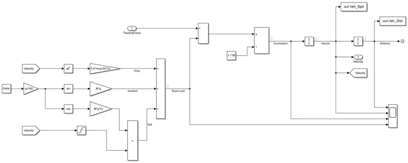
The vehicle dynamics block models the physical relations that defines the motion of the vehicle. It determines the net force acting on the vehicle, by taking into consideration the tractive force generated by the vehicle due to its prime mover and the total resistance forces acting on the vehicle due to its motion. The vehicle can move forward only if the tractive force is greater than the resistance forces or the so-called road load. From the net force, acceleration, velocity and the distance travelled by the vehicle can be determined.
Road load is the total resistance force acting on the vehicle when it is in motion. It is divided into 3 components.
1) Aerodynamic drag (`F_(aero)`): Drag is the resistance force acting on a body in relative motion with respect to a surrounding fluid. As the vehicle moves, it is actually moving against the air in the surrounding. This movement therefore creates a resistance on the vehicle, which is defined as the aerodynamic drag. It is dependent on the density of air (`rho_a`), the frontal surface area of the vehicle (`A_f`), the drag coefficient (`C_d`) and the velocity of the vehicle (v).
`F_(aero) = 1/2*rho_a*A_f*C_d*v^2`
2) Rolling resistance (`F_(roll)`): Rolling resistance or rolling friction is the resistance force acting on the wheels as it rolls over a surface. A vehicle in coasting eventually slows down due to the rolling resistance. It is the product of rolling resistance coefficient (`C_r`) and the normal force acting on the vehicle.
`F_(roll) = C_r*M*g*cos(theta)`
where, `theta` is the angle of the motion of the vehicle with respect to the surface.
3) Resistance due to gradient (`F_(gra)`): If the surface on which the vehicle is moving has a gradient, then the gravitational force acting on the vehicle is the resistance due to that gradient.
`F_(gra) = M*g*sin(theta)`
Road load, `F_r = F_(aero)+F_(roll)+F_(gra)`
Road load is then subtracted from the tractive force , which results in the net force acting on the vehicle. The net force is divided by the equivalent mass of the vehicle, which gives the acceleration of the vehicle. The equivalent mass of the vehicle is the sum of mass of the vehicle and effective mass due to rotational inertial.
`M_(eq) / M = 1 + I_(R)/(M*r_(wh)^2)`
where, `I_R` is the inertial mass of all the rotating components in `kgm^2`, `r_(wh)` is the wheel radius in m. The equivalent mass of a vehicle is normally taken as 1.1 times the actual mass or 10% of the vehicle weight. Therefore `M_(eq) = 1.1*M`.
By integrating the obtained acceleration value, the velocity of the vehicle can be determined and eventually the distance travelled by the vehicle. The obtained velocity serves as the input for the Driver block, where it determines whether the desired velocity has arrived or not. Velocity and distance travelled are transferred to the MATLAB Workspace for post-processing.
Once the engine and vehicle dynamics blocks are modelled, the forward model of the vehicle can be simulated based on the input values initialized using the initialization script. The solver selected for the simulation is ode3 with a fixed step size of 0.01 sec. The simulation time is set as the time at the end of the selected driving cycle. When the simulation is completed without any errors, necessary data from the it will be available in the workspace and post-processing of the data can be done.
Post-processing:
Post-processing is the MATLAB script that is used to analyze the data obtained from the simulation. This script is executed after the simulation is completed and the model data has been loaded into the workspace. Upon execution it takes in the necessary values that are loaded into the MATLAB Workspace, performs some calculations and creates the plots that are required.
MATLAB Script:
%%%%%%%%%%%%%%%%%%%%%%%%%%%%%%%%%%%%%%%%%%%%%%%%%%%%%%%%%%%%%%%%%%%%%
%% Skill-Lync -> Hybrid Drives Development
% Project 1 - Conventional Vehicle Model

%% Post-Processing File
%  File for post-processing the Conventional vehicle simulation model data
close all
clc

%% Renaming variables
Time = out.tout;
Acc_Pdl = out.Acc_Pdl;                     % Accelerator pedal [%]
Brk_Pdl = out.Brk_Pdl;                     % Brake pedal [%]
Gear_Cmd = out.Gear_Cmd;                   % Transmission gear
Trans_In_Spd = out.Trans_In_Spd*30/pi;     % Transmission input speed [rpm]
Trans_Out_Spd = out.Trans_Out_Spd*30/pi;   % Transmission output speed [rpm]
Eng_Trq = out.EngTrq;                      % Engine brake torque [Nm]
Eng_Spd = out.EngSpd*30/pi;                % Engine speed [rpm]
Fuel_Flow_Rate = out.FuelFlowRate;         % Fuel flow rate [g/s]
Eng_Fuel_Consump = out.FuelConsumption;    % Engine fuel consumption [g]
Wheel_Spd = out.Wheel_Spd*30/pi;           % Wheel Speed [rpm]
Veh_Dist = out.Veh_Dist/1000;              % Distance traveled by vehicle [km]
Veh_Spd = out.Veh_Spd*18/5;                % Vehicle speed [kmph]
Veh_desired_Spd = out.Desired_Spd*18/5;    % Desired speed [kmph]


%% Data Analysis
Eng_Pwr = (Eng_Spd*pi/30) .* (Eng_Trq/1000);                     % Engine brake power [kW]
rho_petrol = 0.7197;                                             % Density of petrol [kg/L]
kmpl = Veh_Dist(end)/(Eng_Fuel_Consump(end)/1000/rho_petrol);    % Fuel economy [kmpl]

Drive_Cycle = ["UDDS","HWFET","FTP","US06","NEDC","WLTP"];

if Drive_Cycle_Select == 1
    kmpl_1 = kmpl;
    T = table(Drive_Cycle(1),kmpl_1,'VariableNames',{'Drive cycle','Fuel Economy [km/l]'})

elseif Drive_Cycle_Select == 2
    kmpl_2 = kmpl;
    T = table(Drive_Cycle(2),kmpl_2,'VariableNames',{'Drive cycle','Fuel Economy [km/l]'})

end

%% Plotting vehicle characteristics time trace
% Engine speed, transmission input & output speed and wheel speed
figure('Name','Time trace 1')
hold on
grid on
plot(Time, Eng_Spd,'LineWidth',1,'Color','r')
plot(Time, Trans_In_Spd,'LineWidth',1,'Color','b')
plot(Time, Trans_Out_Spd,'LineWidth',1,'Color','c')
plot(Time, Wheel_Spd,'LineWidth',1,'Color','k')
xlabel('Time [s]')
ylabel('Engine,Transmission In & Out, Wheel Speeds [rpm]')
xlim([0, Time(end)])
title('Time trace of Engine, Transmission input and output and Wheel speed')
legend('Engine Speed','Trans. I/P Speed','Trans. O/P Speed','Wheel Speed')
hold off

% Engine torque, engine power, fuel flow rate and fuel consumption
figure('Name','Time trace 2')
subplot(4,1,1)
plot(Time,Eng_Trq,'LineWidth',1,'Color','k')
grid on
xlim([0, Time(end)])
ylabel('Eng. Brake Torque [Nm]')
legend('Eng. Brake Trq')

subplot(4,1,2)
plot(Time,Eng_Pwr,'LineWidth',1,'Color','k')
grid on
xlim([0, Time(end)])
ylabel('Eng. Brake Power [kW]')
legend('Eng. Brake Pwr')

subplot(4,1,3)
plot(Time,Fuel_Flow_Rate,'LineWidth',1,'Color','r')
grid on
xlim([0, Time(end)])
ylabel('Fuel flow [g/s]')
legend('Fuel flow rate')

subplot(4,1,4)
plot(Time,Eng_Fuel_Consump,'LineWidth',1,'Color','r')
grid on
xlim([0, Time(end)])
ylabel('Fuel Consumption [g]')
xlabel('Time [s]')
legend('Fuel consumption')

% Accelerator & brake pedal positions, gear, vehicle desired & actual speed and distance covered
figure('Name','Time trace 3')
subplot(4,1,1)
hold on
plot(Time, Acc_Pdl, 'linewidth', 1, 'Color', 'black')
plot(Time, Brk_Pdl, 'linewidth', 1, 'Color', 'red')
grid on
xlim([0, Time(end)])
ylabel('Pedal [%]')
legend('Accel','Brake')

subplot(4,1,2)
plot(Time, Gear_Cmd, 'linewidth', 1, 'Color', 'black')
grid on
xlim([0, Time(end)])
ylabel('Gear')
legend('Gear')

subplot(4,1,3)
hold on
plot(Time, Veh_Spd, 'linewidth', 1, 'Color', 'black')
plot(Time, Veh_desired_Spd, 'linewidth', 1, 'Color', 'red')
grid on
xlim([0, Time(end)])
ylabel('Speed [km/h]')
legend('Actual Speed','Desired Speed')

subplot(4,1,4)
plot(Time,Veh_Dist,'LineWidth',1,'Color','k')
grid on
xlim([0, Time(end)])
xlabel('Time [s]')
ylabel('Distance [km]')
legend('Distance covered')

%% Plotting engine operating points on engine fuel map
figure('Name','Engine Operating Points')
hold on
grid on
title('Engine Operating Points','fontsize',12)
p1 = plot(Eng_map_spd*30/pi,Eng_max_trq,'linewidth',2,'color','r');
hold on
p2 = line([Eng_map_spd(end)*30/pi Eng_map_spd(end)*30/pi],[0 Eng_max_trq(end)]);
set(p2,'linewidth',1,'linestyle','--','color','k')
p3 = line([Eng_map_spd(1)*30/pi Eng_map_spd(1)*30/pi],[0 Eng_max_trq(1)]);
set(p3,'linewidth',1,'linestyle','--','color','k')

[c,h] = contour(Eng_map_spd'*30/pi,Eng_map_trq,Eng_fuel_map');
clabel(c,h)
xlabel('Engine Speed [rpm]')
ylabel('Engine Torque [Nm]')
title('Engine Fuel Consumption Map [g/s]')

p4 = plot(Eng_Spd,Eng_Trq,'.','Color','k');
legend([p1 p4],{'Max torque curve','Operating points'})
axis([Eng_map_spd(1)*30/pi Eng_map_spd(end)*30/pi 0 Eng_map_trq(end)])


%% Engine Efficiency Map
figure('Name','Engine Efficiency Map')
hold on
grid on
title('Engine Operating Points','fontsize',12)
p1 = plot(Eng_map_spd*30/pi,Eng_max_trq,'linewidth',2,'color','r');
hold on
p2 = line([Eng_map_spd(end)*30/pi Eng_map_spd(end)*30/pi],[0 Eng_max_trq(end)]);
set(p2,'linewidth',1,'linestyle','--','color','k')
p3 = line([Eng_map_spd(1)*30/pi Eng_map_spd(1)*30/pi],[0 Eng_max_trq(1)]);
set(p3,'linewidth',1,'linestyle','--','color','k')

[c,h] = contour(Eng_map_spd'*30/pi,Eng_map_trq,Eng_eff_map');
clabel(c,h)
xlabel('Engine Speed [rpm]')
ylabel('Engine Torque [Nm]')
title('Engine Efficiency Map')
legend([p1],{'Max torque curve'})
p4 = plot(Eng_Spd,Eng_Trq,'.','Color','k');
legend([p1 p4],{'Max torque curve','Operating points'})
axis([Eng_map_spd(1)*30/pi Eng_map_spd(end)*30/pi 0 Eng_map_trq(end)])
The engine power and fuel economy of the vehicle are calculated in the script. The time trace for:
- engine, transmission input, transmission output and wheel speed are plotted together.
- engine torque, engine power, fuel flow rate and fuel consumption are plotted using subplots.
- accelerator and brake pedal positions, chosen gear, vehicle desired and actual speed, distance travelled are plotted using subplots.
Along with this, the engine operating points are plotted on the engine fuel map and an engine efficiency map is also created.
Results and Inference:
The simulation of forward energy-based fuel consumption model of a conventional vehicle was performed successfully without any errors for both the driving cycles.
Vehicle characteristics:
a) UDDS Cycle
1) Time trace of engine, transmission input, transmission output and wheel speed
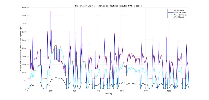
The engine speed coincides almost perfectly with the transmission input speed, this is because the engine is directly connected to the transmission. Transmission reduces the higher engine speed to lower wheel speed and at the same time increases the torque. This depends on the gear ratio of the gears in the transmission system. The effect of the transmission can be seen through the engine and wheel speed. As the engine speed hits peaks above 3000 rpm at various times (maximum speed greater than 4500rpm), the wheel speed has a maximum under 750 rpm. The transmission output speed curve is also finer, with lesser fluctuations in comparison to the input speed.
2) Time trace of engine torque, engine power, fuel flow rate and fuel consumption
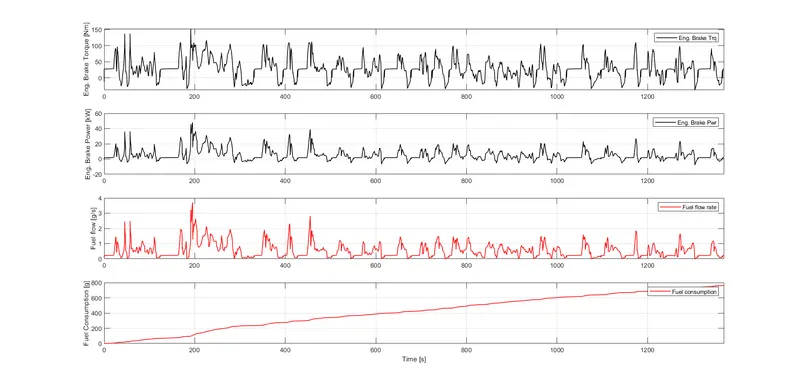
The engine torque has maximum of 152.4102 Nm and a minimum of -37.5416 Nm. Similarly the power produced by the engine varies between 48.0879 kW and -7.9375 kW. The negative torque and power values means the vehicle is decelerating or is in a braking phase. The minimum engine power value is at time 1304.25 sec, which represents a strong deceleration phase in the UDDS cycle. The maximum fuel flow rate is 3.7051 g/s at almost 195 sec of the driving cycle. The UDDS cycle hits its highest velocity around 200 sec. So to accelerate the vehicle to that velocity, the engine needs more torque and for this purpose it takes in more fuel. The maximum torque and power output of the engine also falls near this time. The fuel consumption increases gradually and reaches a maximum of 760.9042 gm.
3) Time trace of accelerator and brake pedal positions, gear, vehicle desired and actual speed, distance travelled
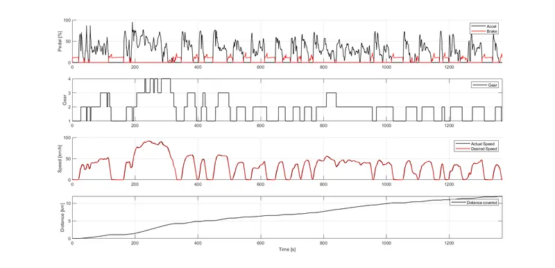
Around the time the UDDS cycle hits the maximum velocity, the accelerator is pressed the maximum. Similarly the brake pedal positions over the cycle are also clear from the above figure. The vehicle has 4 speed automatic transmission. From the above graph the time points of upshifts and downshifts are clearly notable. The vehicle actual speed coincides almost perfectly with the desired speed. How good the actual speed can follow the desired speed is dependant on the controller tuning (controller gains). By choosing the right tuning (using the right values of gain), the accuracy of the controller and its response can be improved. The vehicle covers a distance of almost 12 km during the cycle.
4) Engine operating points on the engine fuel map
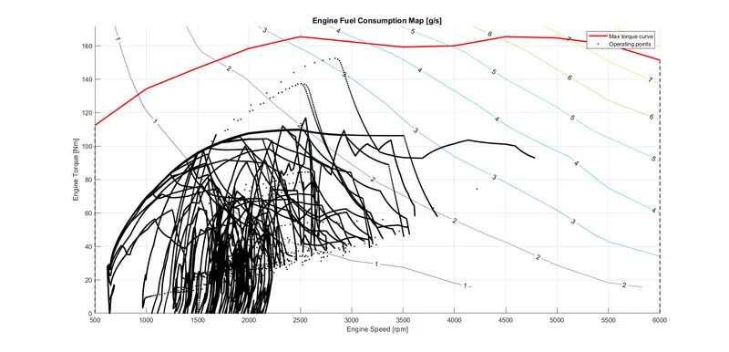
The engine fuel map represents the fuel consumption of the engine at different operating points. The maximum torque curve of the engine is plotted in the map, together with the engine operating points as it traverses through the UDDS cycle. The engine mostly operates under 4000 rpm. It can hit its maximum torque of 165.36 Nm at 2500 rpm and 4500 rpm. But in this driving cycle the maximum required engine torque is 152.4102 Nm at 2838.85 rpm. How the engine operating points changes is visible in the above curve.
5) Engine efficiency map
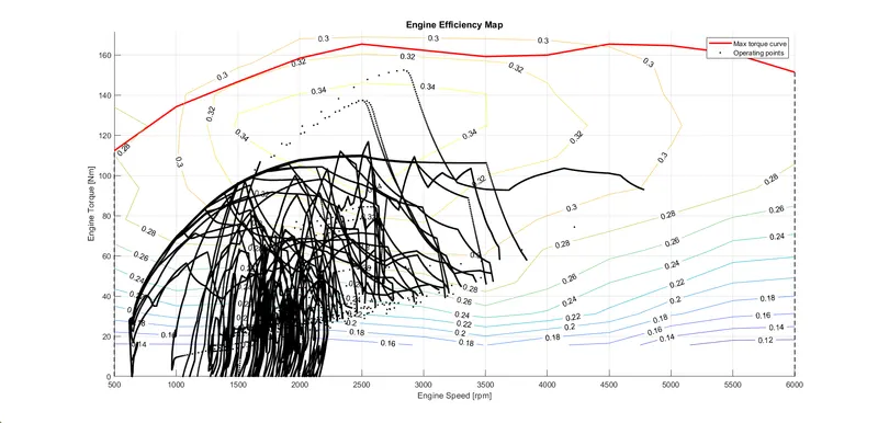
The engine efficiency map represents the regions of engine efficiency. By plotting the operating points on it, it can be understood, in which regions does the engine operate. The engine has maximum efficiency of 34% and when it operates in this region, the fuel consumption will be lowest, as it converts the energy stored in the fuel with higher efficiency. It is also visible that it operates at low efficiency points too at certain time periods, mostly during low torque regions. Higher the load, better the efficiency.
b) HWFET Cycle
1) Time trace of engine, transmission input, transmission output and wheel speed
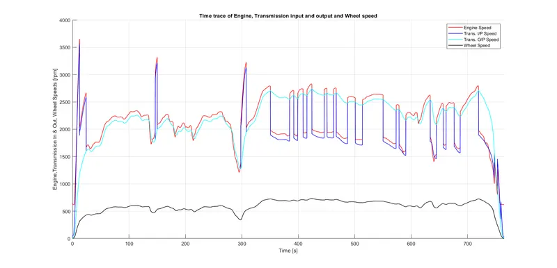
The engine has a maximum speed of 3654.4 rpm in HWFET cycle. The wheel speed also doesn't under go much fluctuations in this cycle, with a maximum of 734.6442 rpm. Transmission input and output speed follows a similar characteristic as in the UDDS cycle.
2) Time trace of engine torque, engine power, fuel flow rate and fuel consumption
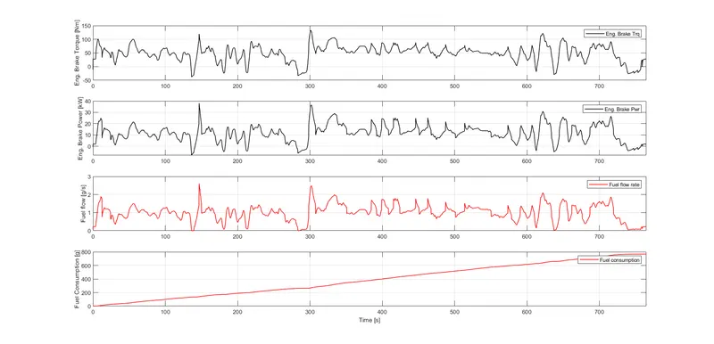
The engine produces a maximum torque of 133.3649 Nm and a maximum power of 38.126 kW. The engine produces a maximum negative power of 8.0547 kW during braking phase. The maximum fuel flow rate into the engine is 2.6101 g/s and over the cycle it consumes around 768.4882 gm fuel, which is actually greater than the total fuel consumed during the UDDS cycle. HWFET cycle is basically a highway cycle and therefore there are less deceleration phases and the fuel flow rate averages around 1 or greater than 1 g/s, which leads to a greater fuel consumption over the whole cycle.
3) Time trace of accelerator and brake pedal positions, gear, vehicle desired and actual speed, distance travelled
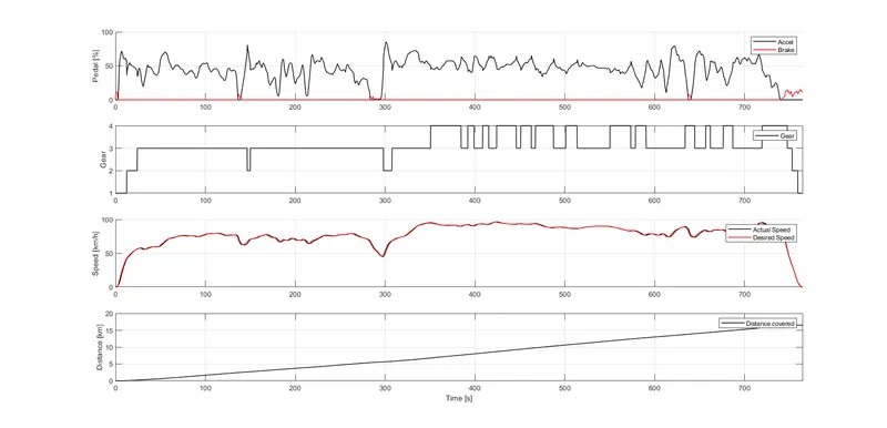
From the time trace of accelerator and brake pedal positions, it is clear that the HWFET cycle has only few braking points (towards the end of the cycle). The changes in gear are also understandable from the above graph. The actual speed of the vehicle closely follows the desired speed and the vehicle covers a total distance of 16.5 km, which is again greater than the UDDS cycle even though it has a greater cycle time.
4) Engine operating points on the engine fuel map
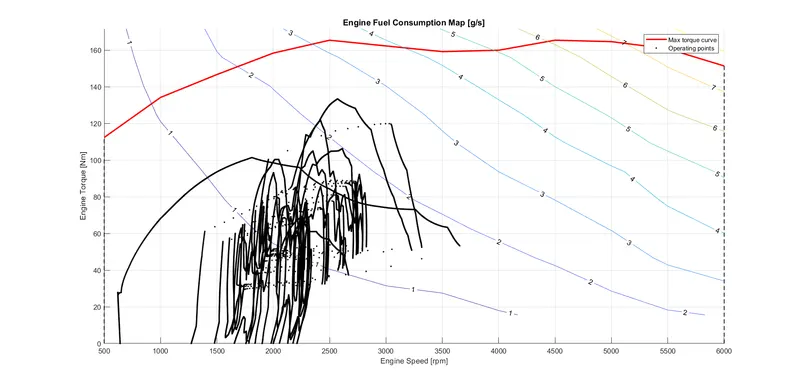
The engine is operating always under 4000 rpm and produces a maximum torque of 133.3649 Nm which is well under the maximum value it can produce. The various engine operating points and the regions of fuel consumption are visible from the above graph.
5) Engine efficiency map
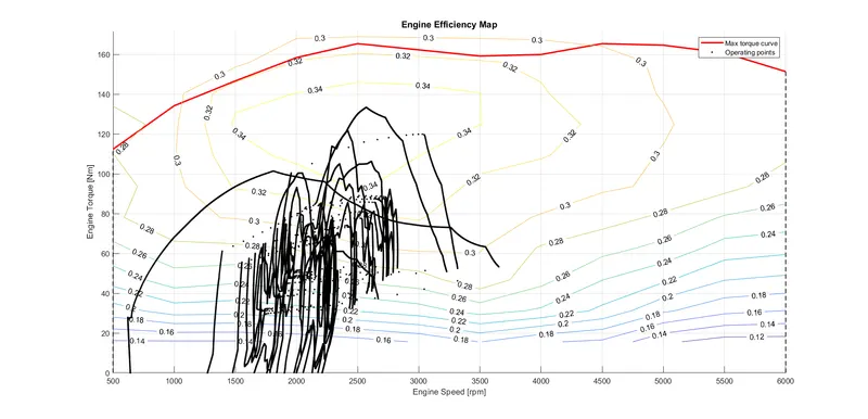
The engine operating points plotted over the efficiency map shows the best operating points of the engine, with the operating points reaching the best efficiency region of 34%. Although most of it lies below this region.
Conclusion:
The main goal of this project was to get familiar with the modeling process, writing scripts in MATLAB, modeling in Simulink, using the MATLAB Workspace to declare and obtain variables, analyzing data and generating plots. All these goals were achieved through this project. Modelling was done in Simulink without any errors and the MATLAB Scripts were used to initialize the data and also to process the output data obtained from the model.
In this project a typical midsize car with a 1.9L engine and a 4-speed automatic transmission was modelled successfully and its various perfomance parameters were analyzed. All the required plots were obtained without errors.