Project 1 - Parsing NASA thermodynamic data

PARSING NASA THERMODYNAMIC DATA

1. Aim
To write a MATLAB code:
• To extract 14 coefficients and then calculate the specific heats, enthalpy and entropy for all the species in the thermodynamic data published by NASA.
• To calculate the molecular weight of each of the species.
• To create plots of specific heat, enthalpy and entropy for the specified local temperature range for each species and to save the plots as images into separate folders automatically.

2. Theory
Thermodynamical properties are important factors in all the combustion related problems. In 1961 Frank Zeleznik and Sanford Gordon invented a method for performing a simultaneous regression of the thermochemical properties in order to approximate more than one property with a single polynomial and ended up with the famous NASA 7 term polynomials first
published by Zeleznik and Gordon (1962) and McBride et al. (1963). These polynomials have evolved a lot over time and are widely accepted and extensively used in wide variety of applications. These polynomials are provided in large databases and contains coefficients for more than 1300 species. A major problem with the database is that it is provided in a text file
[1].
The NASA polynomials have the form:

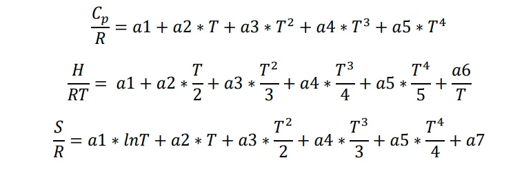
Where a1, a2, a3, a4, a5, a6, and a7 are the numerical coefficients supplied in NASA thermodynamic files. Each species has 14 different coefficients of which the first 7 are the coefficients for the high temperature range and the next 7 are the coefficients for the low temperature range. The temperature ranges for each species are mentioned alongside the species
entry. By extracting the coefficients out from the data file and using the above-mentioned formulas, specific heat, enthalpy and entropy of each of the species over the specified temperature range can be determined [2].

3. Inputs
The only input for the program is the thermodynamic data file containing all the coefficients for different species.

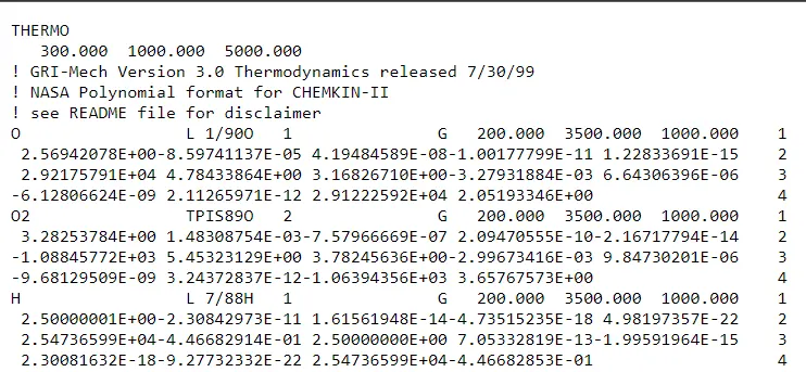
Figure 1 Screenshot of the data file

In the data file (above figure), lines that begin with an exclamation (!) are comment lines, which here form the header of the file, and are not necessary part of the program. The species entries begin right after the header. In the first line of the species entry, the local temperature range for the species are mentioned. From the second line after the species entry begins the coefficients. The first 7 numbers starting from the second line (five from the second line and the first two from the third line) are the seven coefficients for the high temperature range (temperatures lying above the middle value as specified in the local temperature range). The remaining seven are the coefficients for the low temperature range.

4. Program
The MATLAB program consists of a main body and 5 functions:

1. Function 1 – linecount: to calculate the number of lines in the entire data file.
2. Function 2 – specific_heat: to determine the specific heat of the species depending on the temperature.
3. Function 3 – enthalpy: to determine the enthalpy of the species depending on the temperature.
4. Function 4 – entropy: to determine the entropy of the species depending on the temperature.
5. Function 5 – molecular_wt: to calculate the molecular weight of each of the species.

The main body of the program begins with assigning the universal gas constant to a variable, followed by opening the thermodynamic data file (using ‘fopen’) and assigning it to a variable. The lines of the opened file are then read using ‘fgetl’. This command moves line by line each time it is called. From Figure 1, the second line of the file contains three numbers, which are the global temperature ranges for all the species in the data file. These are first extracted out by storing them in a char array and then splitting the char array using ‘strsplit’, where strsplit looks for spaces ‘ ’ in the char array and splits the array based on the spaces. The values that are split are stored in a cell array and these are then extracted out and stored as numerical values(using ‘str2num’) in a new variable. The values are then finally classified as the global – low, mid and high temperatures.

In order to understand what the contents of the data file are, the number of lines in the file are counted using the function ‘linecount’. Linecount uses the lines of the file as input and then using a while loop check whether the line that is read is a character array or not. If the input contains a character array the loop increments a counter variable. The loop ends when it is not able to find a character array. So, using this function the total number of lines in the file can be counted. Now that all the lines of the file are read, the position of fgetl needs to be resetted. Using the ‘frewind’ command the file position indicator can be moved to the beginning of the open file. After that using a for loop all the lines of the data file are again read and are stored as characters into a cell array. The user can now open the cell array to look through the contents of the given data file right from the program.

In order to extract the coefficients, it is important to determine the number of species in the data file. By going through the cell array containing all the elements of the data file, it was clear that the first 5 lines contain the header information, and the last 3 lines include an “END” and empty spaces. It was also understood that every 4th line contains a species (see Figure 1 for further clarification). Since the total number of lines are known and using the information obtained from the cell array, it was possible to calculate the number of species in the data file. It is displayed in the command window when the program is executed.

Now begins the extraction of the necessary information from the data file. Again, the file position indicator is reset using frewind and using a loop the first five lines or the header information is skipped. From there a loop is used to do repeat the same processes for all the species in the data file. In the species entry line, the first element is always the species name
(see Figure 1). By using strsplit and looking for spaces the entry line can be split up and from this the element name can be extracted out and stored as a character. The element name is then displayed during execution. Now to identify the local temperature range, the ‘strfind’ command is used. It is clear from Figure 1 that the local temperature range consists of decimal values. So strfind is used to search for dots (“.”) in the line and it returns the position of these dots. Based on the position of these dots, the temperature values can be determined. Here str2num is used to convert the string (the entry line) to numerical values. The local – low, mid and high temperatures can now be extracted out to corresponding variables.

Now that all the information from the entry line has been extracted, the program moves onto the lines containing the coefficients. In the data file the coefficients of each species are written in 3 lines. The program reads the file line by line and extracts the coefficients contained in each line. From Figure 1, it is understood that all the coefficients or all the number in the 3 lines after the species entry contains an “E” to represent the 10^th power. It is the only common element in all the coefficients. Using strfind the position of E in a line can be determined and based on the position of the exponent, the whole coefficient can be determined. The string is then converted to a numerical value and is stored in a corresponding variable. The line after the species entry is extracted using fgetl and stored as line_1, similarly line_2 and line_3, the subsequent lines containing the coefficients are also extracted out. The process using strfind is performed on all these lines to take out all the coefficients. These are then stored in variables a1, a2, a3……. a14.

After the coefficients are successfully extracted out, the specific heat, enthalpy and entropy of the species are calculated using corresponding MATLAB functions.

• Specific heat calculation:

A MATLAB function called ‘specific_heat’ is initialised for this purpose. The inputs of this function are the determined coefficients (a1 – a5, a8 – a12, as all the coefficients are not needed for calculating the specific heat), the determined local- low, mid and high temperatures and the universal gas constant. Based on the temperatures, a temperature range is established using linspace with 500 divisions. Now using a loop, the specific heat values for the entire temperature can be calculated. The condition for the calculation is that, if the temperature is above the local mid temperature, the high temperature coefficients (a1 – a7) are used for the calculation and if it is below the local mid temperature, the low temperature coefficients (a8 – a14) are used. The function outputs the specific heat, which is then stored as a row vector cp, where each row gives the value for the corresponding element.

• Enthalpy calculation:

A MATLAB function called ‘enthalpy’ is initialised for this purpose. The inputs of this function are the coefficients (a1 – a6, a8 – a13), the local temperature values and the universal gas constant. A temperature range is established and based on the condition, as the one mentioned in the above calculation, the enthalpy values for the established temperature range is determined. The function outputs the enthalpy values, which are stored in a row vector h.

• Entropy calculation:

A MATLAB function of the name ‘entropy’ is initialised for this calculation. The inputs of this function are all the determined coefficients (a1 – a14), the local temperature values and the universal gas constant. The logic of this calculation is same as the ones used in the previous functions. A temperature range is created and based on the temperature values, the low or high temperature coefficients are used for calculating the entropy values of the species. The function outputs the entropy values for the entirety of the temperature range and stores them as a row a vector s.

• Molecular weight calculation:

A MATLAB function – ‘molecular_wt’ is initialised for this calculation. The input for this function is the species’ name which is stored as a character array/string. Since the entire data file contains only 5 elements, namely – H, C, N, O, and Ar, they are initialised as characters in a cell array and their corresponding masses are initialised as a column vector. A new variable is also initialised to store the total molecular weight of the entire species. The function uses nested loops to traverse through the string of species name as well as through the initialised element names. It uses ‘strcmp’ in an ‘if ’ statement to compare the characters from the input to the elements and whenever a match is found it stores the element mass in a new variable and adds this to the total molecular weight of the entire species. To determine the number of moles of a particular element, each character of the species name is also compared to numbers between 0 – 9 in an ‘elseif ’ statement. If a match occurs, the number is extracted from the string and converted into a numerical value (using str2num) and is stored in a variable. It is then multiplied with the molar mass of the element, but here number of moles minus 1 is used, because in the first if statement the molar mass of the element is added once to the total mass of the species. So, in the second statement, it is only necessary to have the number of moles minus 1. In this way the total molecular weight of each of the species in the data file can be calculated. This function is only applicable to the given data file and cannot be used for a general application. The function outputs the total molecular weight and is stored in a variable M, which gets overwritten during every iteration. The main body of the program outputs the molecular weight of each of the species in each iteration.

The next part of the program focusses on creating the plots of specific heat, enthalpy and entropy vs local temperature range as well as creating folders for saving these plots. As the per the aim of the project, the plots that are created for each species must be stored into separate folders automatically. Therefore, the program needs to create folders for each species during each iteration. To create a folder the predefined MATLAB command ‘mkdir’ can be used. Its input is the location of the folder that needs to be created. By default, mkdir creates folders at the location where the MATLAB code is saved to. The main folder name is given as ‘Plots’ and the subfolders are named as the species name. So, during each iteration of the loop a folder in the name of the species will get created inside a main folder called Plots. The location of the subfolders is specified using ‘fullfile’ command.

A total of three plots,

1. Specific heat vs Temperature
2. Enthalpy vs Temperature
3. Entropy vs Temperature

needs to be created for each of the species after the execution of the program. The temperature range for each of these plots are the local temperature ranges that are extracted out during the beginning of the loop. The plot command is then used to create the corresponding plots in the form of 3 different figures. The visibility of the plot is set as off, to hide the plots during execution. The necessary axis labels and titles are assigned to each of the plots. Now to save them to the folders created, ‘saveas’ command is used. Using the command ‘gcf ’ the frame of the image is captured, using fullfile the save location and name of the figure file is specified and then using saveas, it is saved to the desired location. Each of the created folders will contain the plots after executing the program.

5. Results

The program was able to extract the 14 different coefficients and calculate the specific heat, enthalpy and entropy for all the species mentioned in the thermodynamic data published by NASA. The specific heat, enthalpy and entropy vs temperature plots were obtained and were also saved in separate folders after the program execution. The molecular weight of each of the elements were also displayed as output in the command window.

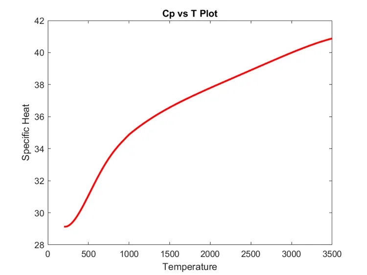
Figure 2 Specific heat vs Temperature of O2

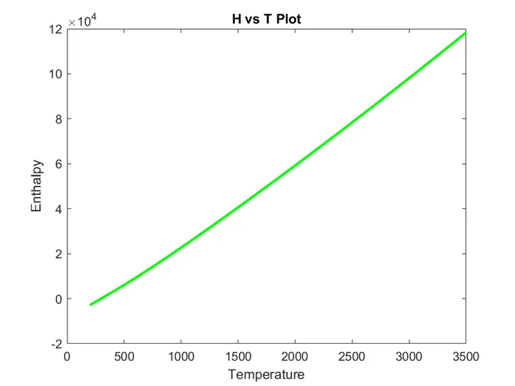
Figure 3 Enthalpy vs Temperature of O2

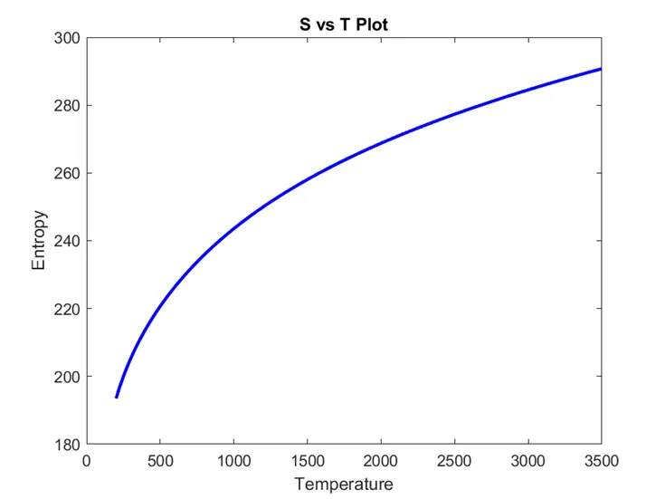
Figure 4 Entropy vs Temperature of O2

Figure 5 Folders created for each species after execution

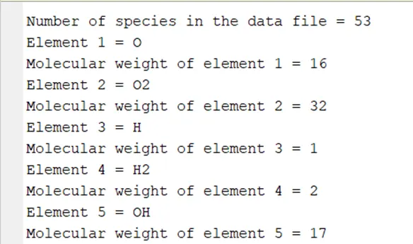
Figure 6 Molecular weight displayed in the command window

6. Inference

The focus of this project was to understand how to parse through a data file and extract the necessary information from it. Based on the extracted data certain calculations needed to be done and finally plots were created, which were then saved to specific folders.

Through this project, the understanding of:

• file parsing and the commands involved (fopen, fgetl…etc),
• initialising and calling MATLAB functions,
• creating folders using MATLAB (mkdir, fullfile…etc),
• saving figures to a particular folder (saveas)

and how to apply them in a program were achieved.

7. References

[1] https://myengineeringworld.net/2013/10/excel-thermochemical-nasa-polynomials-burcat.html

[2] http://combustion.berkeley.edu/gri-mech/data/nasa_plnm.html

[3] http://combustion.berkeley.edu/gri-mech/version30/files30/thermo30.dat

Original report: https://drive.google.com/file/d/1N3ORs51VDfn-isc841AM6QxRkTs2Xxul/view?usp=sharing

MATLAB code

Main body:

% Parsing NASA thermodynamic data
close all
clear all
clc

% Inputs
R = 8.314; % Universal gas constant
th_file = fopen('THERMO.dat','r') % Opening the data file
fgetl(th_file); % Reading the first line
tline = fgetl(th_file) % Reading the second line and storing it in a new variable
h_temp = strsplit(tline,' ') % Splitting the string

% Extracting out the values from the splitted string and storing it as numerical values
for i = 2:length(h_temp)
    l1(i-1) = str2num(h_temp{i}) 
end

% Classifying the extracted values
global_low_temp = l1(1);
global_mid_temp = l1(2);
global_high_temp = l1(3);

% Counting the number of lines in data file
n = linecount(th_file)

frewind(th_file)
for i = 1:n
    line = fgetl(th_file);
    C{i} = char(line);
    C = C';
end

% Calculating the number of species (or elements) in the data file
% As per the character file C, the first 5 lines belong to the header and the
% last 3 lines include an 'END' and empty spaces

N = (n-3-5)/4; % Every 4th line contains a species
disp(['Number of species in the data file = ',num2str(N)])

% Skipping the header lines
frewind(th_file)
for i = 1:5
    tline = fgetl(th_file);
end

%mkdir Plots
for i = 1:N
    % Extracting the species name from the data file
    line = fgetl(th_file);

    % Species identification
    S = strsplit(line,' ');
    species = char(S(1));

    % Local temperature identification
    T = strfind(line,'.'); 
    local_low_temp = str2num(line(T(1)-4:T(1)+3)); % Check if it is possible to identify the temp from the string and get the position
    local_high_temp = str2num(line(T(2)-4:T(2)+3));
    local_mid_temp = str2num(line(T(3)-4:T(3)+3));
    temp_range = linspace(local_low_temp,local_high_temp,500);

    % Displaying the element name
    disp(['Element ',num2str(i),' = ',species])

    % Extracting the coefficients
    % In the data file, the coefficients for each species are written in 3
    % lines
    line_1 = fgetl(th_file); % Reads the first line of coefficients
    l1 = strfind(line_1,'E');
    a1 = str2num(line_1(1:l1(1)+3));
    a2 = str2num(line_1(l1(1)+4:l1(2)+3));
    a3 = str2num(line_1(l1(2)+4:l1(3)+3));
    a4 = str2num(line_1(l1(3)+4:l1(4)+3));
    a5 = str2num(line_1(l1(4)+4:l1(5)+3));

    line_2 = fgetl(th_file); % Reads the second line of coefficients
    l2 = strfind(line_2,'E');
    a6 = str2num(line_2(1:l2(1)+3));
    a7 = str2num(line_2(l2(1)+4:l2(2)+3));
    a8 = str2num(line_2(l2(2)+4:l2(3)+3));
    a9 = str2num(line_2(l2(3)+4:l2(4)+3));
    a10 = str2num(line_2(l2(4)+4:l2(5)+3));

    line_3 = fgetl(th_file); % Reads the third line of coefficients
    l3 = strfind(line_3,'E');
    a11 = str2num(line_3(1:l3(1)+3));
    a12 = str2num(line_3(l3(1)+4:l3(2)+3));
    a13 = str2num(line_3(l3(2)+4:l3(3)+3));
    a14 = str2num(line_3(l3(3)+4:l3(4)+3));
    % a1 - a7 high temp. coefficients
    % a8 - a14 low temp. coefficients

    % Calculating specific heat
    cp(i,:) = specific_heat(a1,a2,a3,a4,a5,a8,a9,a10,a11,a12,local_low_temp,local_high_temp,local_mid_temp,R);

    % Calculating enthalpy
    h(i,:) = enthalpy(a1,a2,a3,a4,a5,a6,a8,a9,a10,a11,a12,a13,local_low_temp,local_high_temp,local_mid_temp,R);
    
    % Calculating entropy
    s(i,:) = entropy(a1,a2,a3,a4,a5,a6,a7,a8,a9,a10,a11,a12,a13,a14,local_low_temp,local_high_temp,local_mid_temp,R);

    % Calculating molar mass
    M = molecular_wt(species);
    disp(['Molecular weight of element ',num2str(i),' = ',num2str(M)]) % Displaying the molecular weight

    % Creating folders for saving plots
    main_folder = 'Plots';
    sub_folder = species;
    mkdir(fullfile(main_folder,sub_folder));

    % Plots
    figure(1)
    plot(temp_range,cp(i,:),'Color','r','LineWidth',2)
    set(figure(1),'visible','off') % To hide the figures after plotting
    xlabel('Temperature')
    ylabel('Specific Heat')
    title('Cp vs T Plot')
    saveas(gcf,fullfile(main_folder,sub_folder,('Specific Heat.png')))

    figure(2)
    plot(temp_range,h(i,:),'Color','g','LineWidth',2)
    set(figure(2),'visible','off')
    xlabel('Temperature')
    ylabel('Enthalpy')
    title('H vs T Plot')
    saveas(gcf,fullfile(main_folder,sub_folder,('Enthalpy.png')))

    figure(3)
    plot(temp_range,s(i,:),'Color','b','LineWidth',2)
    set(figure(3),'visible','off')
    xlabel('Temperature')
    ylabel('Entropy')
    title('S vs T Plot')
    saveas(gcf,fullfile(main_folder,sub_folder,('Entropy.png')))
end

Function 1 - linecount

% Function to count the number of lines

function [n] = linecount(file)
n = 0;
tline = fgetl(file);
while ischar(tline)
  tline = fgetl(file);
  n = n+1;
end

Function 2 - specific_heat

% Function to calculate the specific heat

function [cp,TR] = specific_heat(a1,a2,a3,a4,a5,a8,a9,a10,a11,a12,local_low_temp,local_high_temp,local_mid_temp,R) 

TR = linspace(local_low_temp,local_high_temp,500);
for i = 1:length(TR)
    if TR(i) >= local_mid_temp
        cp(i) = R*(a1 + a2*TR(i) + a3*TR(i)^2 + a4*TR(i)^3 + a5*TR(i)^4);
    else 
        cp(i) = R*(a8 + a9*TR(i) + a10*TR(i)^2 + a11*TR(i)^3 + a12*TR(i)^4);
    end
end
end

Function 3 - enthalpy

% Function to calculate enthalpy

function [h] = enthalpy(a1,a2,a3,a4,a5,a6,a8,a9,a10,a11,a12,a13,local_low_temp,local_high_temp,local_mid_temp,R)

TR = linspace(local_low_temp,local_high_temp,500);
for i = 1:length(TR)
    if TR(i) >= local_mid_temp
        h(i) = R*TR(i)*(a1 + a2*TR(i)/2 + a3*TR(i)^2/3 + a4*TR(i)^3/4 + a5*TR(i)^4/5 + a6/TR(i));
    else
        h(i) = R*TR(i)*(a8 + a9*TR(i)/2 + a10*TR(i)^2/3 + a11*TR(i)^3/4 + a12*TR(i)^4/5 + a13/TR(i));
    end
end
end

Function 4 - entropy

% Function to calculate entropy

function [s] = entropy(a1,a2,a3,a4,a5,a6,a7,a8,a9,a10,a11,a12,a13,a14,local_low_temp,local_high_temp,local_mid_temp,R)

TR = linspace(local_low_temp,local_high_temp,500);
for i = 1:length(TR)
    if TR(i) >= local_mid_temp
        s(i) = R*(a1*log(TR(i)) + a2*TR(i) + a3*TR(i)^2/2 + a4*TR(i)^3/3 + a5*TR(i)^4/4 + a7);
    else
        s(i) = R*(a8*log(TR(i)) + a9*TR(i) + a10*TR(i)^2/2 + a11*TR(i)^3/3 + a12*TR(i)^4/4 + a14);
    end
end
end

Function 5 - molecular_wt

% Function to calculate the molecular weight of species in data file
% The data file contains the elements - H,C,O,N,Ar

function [Mw] = molecular_wt(species)

% Assigning the molar mass of each element

elements = {'H';'C';'O';'N';'A'}; % Elements as a cell array
Mm = [1;12;16;14;40]; % Mass of elements

Mw = 0; % Initialising the molecular weight
i = 1;
while i <= length(species)
    for j = 1:length(elements)
        if strcmp(species(i),elements(j)) == 1
                m = Mm(j);
                Mw = Mw + m;
                break
        elseif (species(i) >= '0') & (species(i) <= '9')
                n = str2num(species(i));
                Mw = Mw + m*(n-1);
                break        
        end
    end
    i = i+1;
end
end