Project 1

Aim: Deals with the development of a forward energy-based fuel consumption model of a conventional vehicle.

objectives:

Tabulate the fuel economy numbers (kmpl) for UDDS and HWFET cycle. This forms the baseline numbers for comparing with the future hybrid version.
b. Plot the time trace for engine, transmission input, transmission output and wheel speed on one plot.
c. Plot engine torque, engine power, fuel rate and fuel consumption using subplots.
d. Plot accelerator and brake pedal, gear command, vehicle desired and actual speed, vehicle distance using subplots.
e. Plot the engine operating points on the engine fuel map.
f. Write down appropriate brief comments on each of these plots, describing the vehicle behavior throughout the drive cycle.
g. Generate the plots for both drive cycles

Conventional vehicle:

A conventional vehicle refers to a vehicle that is powered by an internal combustion engine (ICE), typically fueled by gasoline (petrol) or diesel. These vehicles have been the standard mode of transportation for over a century and remain widely used globally.A conventional vehicle refers to a vehicle that is powered by an internal combustion engine (ICE), typically fueled by gasoline (petrol) or diesel. These vehicles have been the standard mode of transportation for over a century and remain widely used globally.

Key Components of a Conventional Vehicle:

1. Internal Combustion Engine (ICE)

   • Converts chemical energy from fuel into mechanical energy.

   • Types: Spark ignition (gasoline) or compression ignition (diesel).

2. Fuel System

   • Stores and supplies fuel to the engine.

   • Includes fuel tank, fuel pump, and injectors/carburetor.

3. Transmission System

   • Transfers power from the engine to the wheels.

   • Can be manual, automatic, or semi-automatic.

4. Exhaust System

   • Removes and treats engine emissions (CO₂, NOx, particulates).

   • Includes catalytic converters and mufflers.

5. Cooling System

   • Maintains optimal engine temperature using coolant, radiator, and fans.

6. Lubrication System

   • Reduces friction and wear of moving engine parts using oil.

7. Electrical System

• Powers lights, starter motor, infotainment, and accessories.

• Includes an alternator and 12V battery.

Main Subsystems of a Forward Model in Simulink for a Conventional Vehicle:
1. Driver Model

• Generates throttle and brake commands based on speed reference.

• Often implemented using a PI controller.

2. Powertrain Model

Includes:

• Engine model: Converts throttle input to torque using maps (e.g., torque vs. RPM vs. throttle).

• Transmission model: Maps engine speed to wheel speed using gear ratios.

• Clutch or torque converter (depending on manual or automatic).

• Differential and final drive: Transfers torque to the wheels.

3. Vehicle Dynamics Model

• Converts wheel torque into vehicle acceleration.

• Accounts for:

  • Rolling resistance

  • Aerodynamic drag

  • Gradient resistance (road slope)

  • Vehicle mass

Uses Newton’s second law:

$$F_{\text{net}} = m \cdot a = F_{\text{drive}} - F_{\text{resistances}}$$Fnet​=m⋅a=Fdrive​−Fresistances​

4. Wheel and Tire Dynamics

• Rotational inertia of wheels.

• Tire slip and grip modeling if needed (e.g., using Magic Formula).

5. Environment

• Road slope

• Wind

• Ambient conditions (optional)

6. Fuel Consumption Model

• Based on engine torque and speed.

• Uses fuel map or brake-specific fuel consumption (BSFC) data.

A fuel consumption model calculates the rate of fuel usage or total fuel consumed by an internal combustion engine (ICE) vehicle based on parameters like engine speed, engine torque, and throttle position. This model is crucial for performance analysis, emissions estimation, and control strategies.

1. Map-Based Model (BSFC Map Method)

BSFC = Brake Specific Fuel Consumption
Represents fuel efficiency of an engine in grams of fuel per kilowatt-hour (g/kWh).

Inputs:

• Engine torque (T_engine)

• Engine speed (ω_engine)

Process:

• Use a BSFC map (lookup table) indexed by torque and speed.

• Calculate fuel power:

  $$P_{\text{fuel}} = \text{BSFC}(T, \omega) \times P_{\text{engine}} / 3600$$Pfuel​=BSFC(T,ω)×Pengine​/3600

• Fuel flow rate:

  $$\dot{m}_{\text{fuel}} = \frac{\text{BSFC} \times T_{\text{engine}} \cdot \omega_{\text{engine}}}{\eta \cdot 3600}$$m˙fuel​=η⋅3600BSFC×Tengine​⋅ωengine​​

Where:

• $T \cdot \omega$T⋅ω = Engine power

• $\eta$η = Mechanical efficiency

• 3600 = Seconds per hour (unit conversion)

MATLAB script:

%%%%%%%%%%%%%%%%%%%%%%%%%%%%%%%%%%%%%%%%%%%%%%%%%%%%%%%%%%%%%%%%%%%%%

%% Skill-Lync -> Hybrid Drives Development

% Project 1 - Conventional Vehicle Model

% By - Anas K Y

% Description:

%% Initialization File

% Initialization file for loading the variables for the Conventional vehicle simulation model

%% Vehicle Parameters

M = 1500; % Vehicle weight [kg]

Cr = 0.015; % Rolling resistance coefficient

Rw = 0.35; % Rolling radius [m]

Cd = 0.33; % Drag coefficient

Af = 2; % Frontal area [m2]

rhoa = 1.225; % Air density [kg/m3]

Vwind = 0; % Wind velocity [kmph]

g = 9.81; % Gravitational acceleration [m/s2]

theta = 0; % Slope [deg]

myu_road_tire = 1; % Coefficient of friction between tire - road interface

%% Powertrain Parameters

FDR = 3.73; % Final Drive Ratio / Diff Ratio

DiffEff = 0.99; % Differential efficiency (assumed independent of operating conditions)

NumGear = 4; % Number of gears in transmission

TransGear = [1:NumGear]; % Transmission Gears

TransRatio = [3.06, 1.62, 1, 0.7]; % Corresponding Transmission ratios

TransEff = 0.90; % Transmission efficiency (assumed independent of operating conditions)

TC_SR = [0, .5, .6, .7, .8, .87, .92, .94, .96, .97, 1]; % Torque Converter Speed Ratio (Matlab default) -> TurbSpd/PumpSpd

TC_TR = [2.232, 1.5462, 1.4058, 1.2746, 1.1528, 1.0732, 1.0192, 1, 1, 1, 1]; % Torque Converter Torque Ratio (Matlab default) -> TurbTrq/PumpTrq

TC_Cf = 1e-4 * [.72558, .66322, .63463, .59042, .51331, .4144, .29287, .22444, .12186, .04386, 0]; % Torque Converter Capacity Factor (Matlab default) -> PumpTrq/PumpSpd^2 [Nm/rpm^2]

load ('Engine_data_1_9L_Saturn_95kW')

load ('Trans_Shift_map')

%% Driver Parameters

Kp = 10; % P gain for driver PI model

Ki = 1; % I gain for driver PI model

Drive_Cycle_Select = 2; % Drive cycle selection

% Drive cycle values in m/s

if Drive_Cycle_Select == 1

load UDDS;

elseif Drive_Cycle_Select == 2

load HWFET;

elseif Drive_Cycle_Select == 3

load FTP;

elseif Drive_Cycle_Select == 4

load US06;

elseif Drive_Cycle_Select == 5

load NEDC;

elseif Drive_Cycle_Select == 6

load WLTP;

end

time_end = cyc_time(end);

vel_end = cyc_vel(end);

Simulink model:

The "project_init_file.m" file is used to load the required data to built the simulink model.

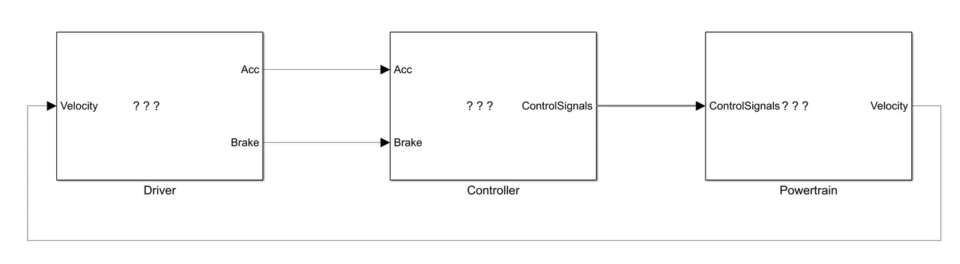
Driver:

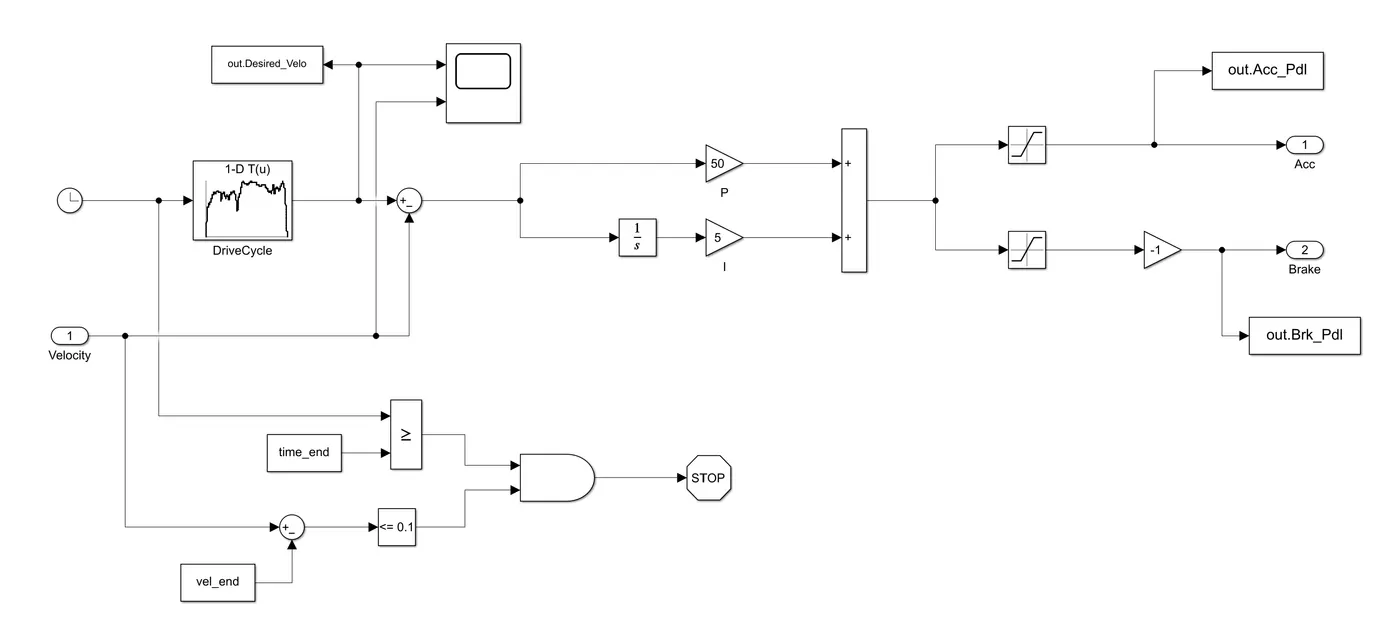
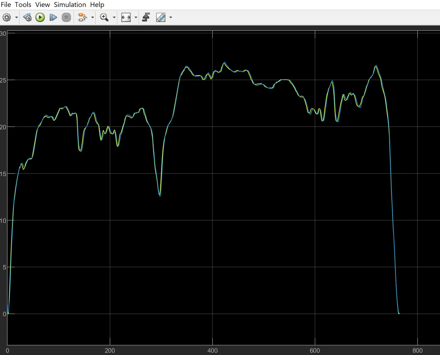
It is modeled using a ‘Driver’ block, which is a basic PI controller that generates accelerator and brake pedal outputs to match the desired and actual vehicle speeds. In this we use drive cycles fro the based on these results of fuel consumption and emissions the vehicle gets certified and it also forms a basis of uniform asessment. It is based on time, velocity then its all integrate and creates output accelration pedal and brake pedal.

graph from driver block:

2.Controller Block:
It consists of three primary control units: the Engine Control Unit (ECU), the Transmission Control Unit (TCU), and the Brake Control Unit (BCU). These subsystems receive inputs from the driver model, which typically outputs throttle (acceleration) and brake commands based on a reference speed (such as from a drive cycle).

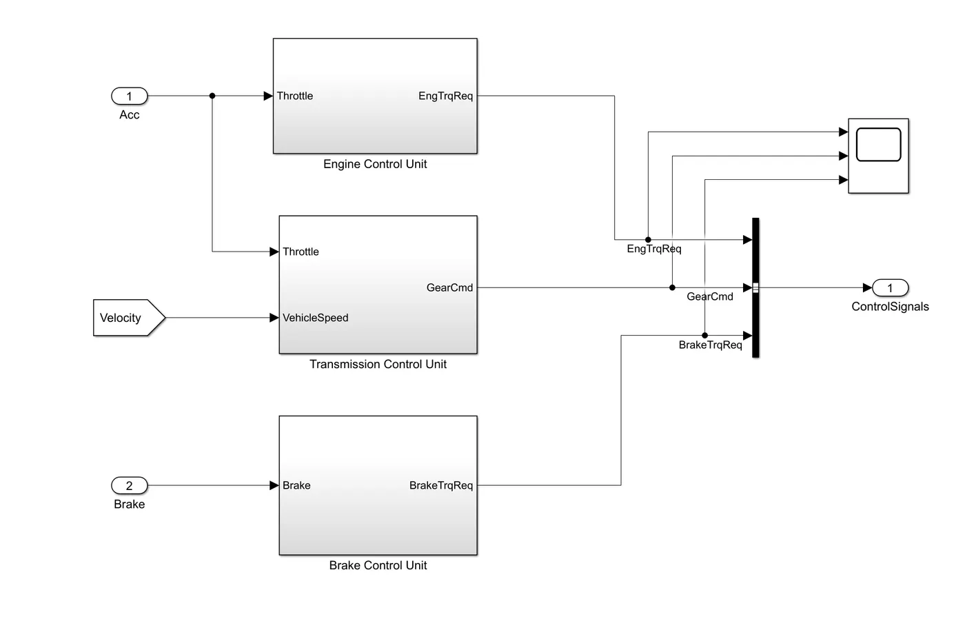
1.Engine control unit:
The Engine Control Unit takes the throttle input from the driver block and translates it into an engine torque request (EngTrqReq). This conversion is often done using engine maps or lookup tables that relate throttle position and engine speed to the desired output torque. The ECU may also include logic for idle torque handling and torque limiting based on engine constraints.

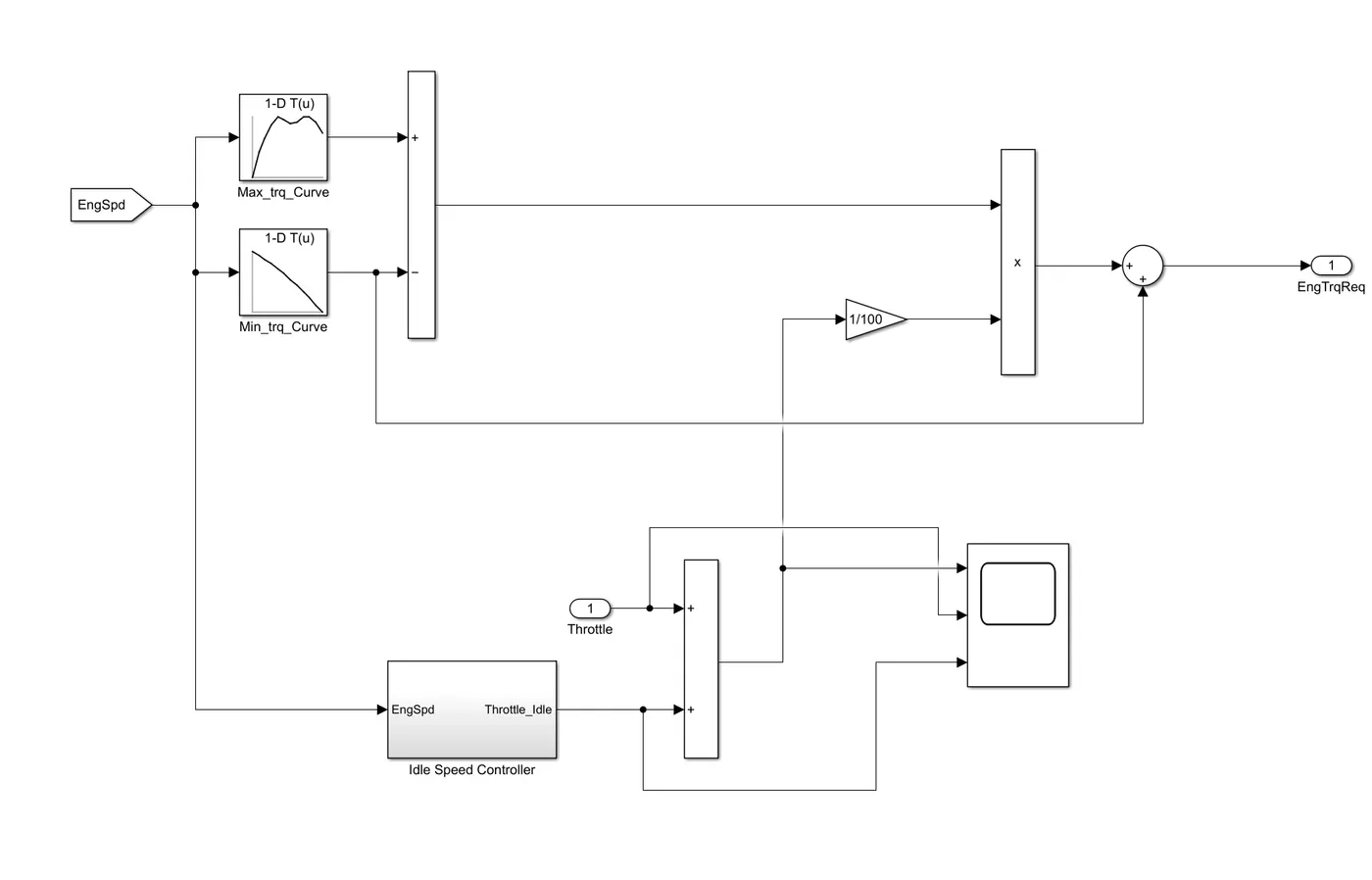
In this control model We use engine control unit in that give input Engine speed through creating look up table. in that table we give input Maximum torque and map speed then also create 2nd look up trable in that give input ct torque and map speed then it substracts and multiplied. the engine speed also give to ideal contro speed to integrate from this we meet output of engine required torque.

2.Transmission:

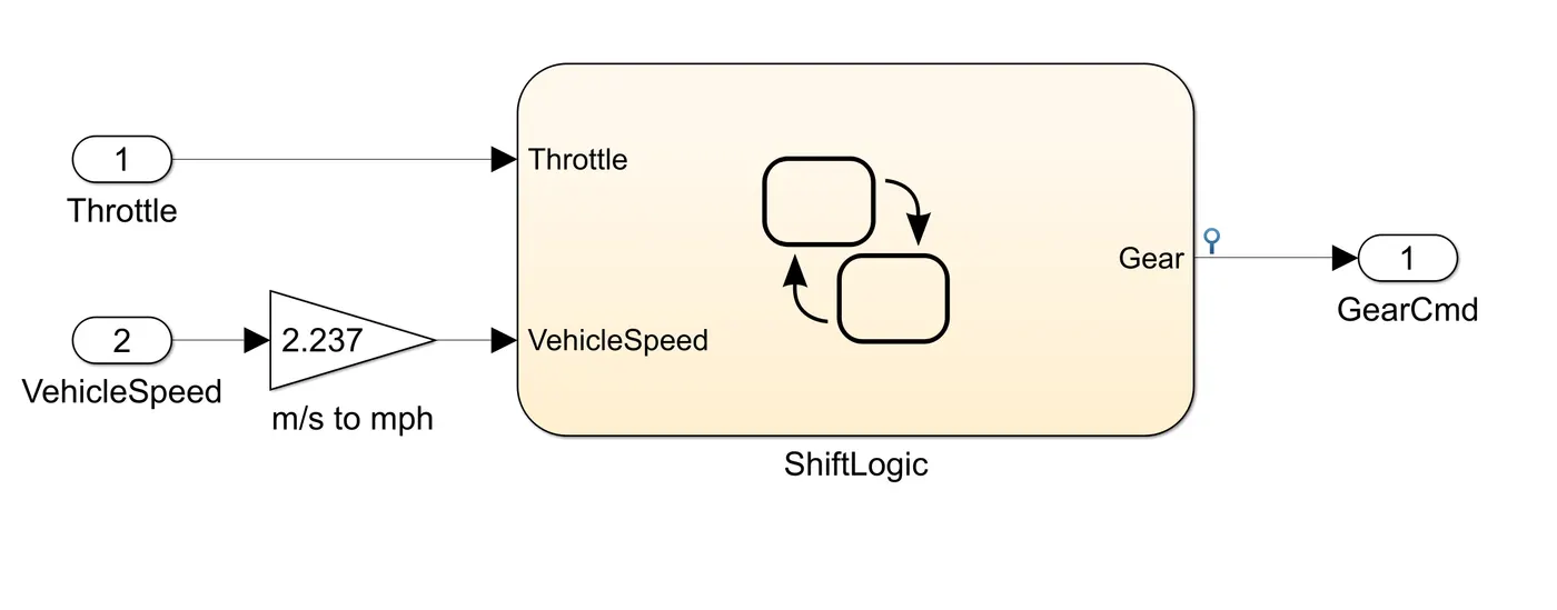
In this unit we create steadfy flow variable state for controlling of gears of vehicle as in ascending and descending order with respect to time, speed, distance. and give input to this steady state is vehicle speed in m/s to mph.

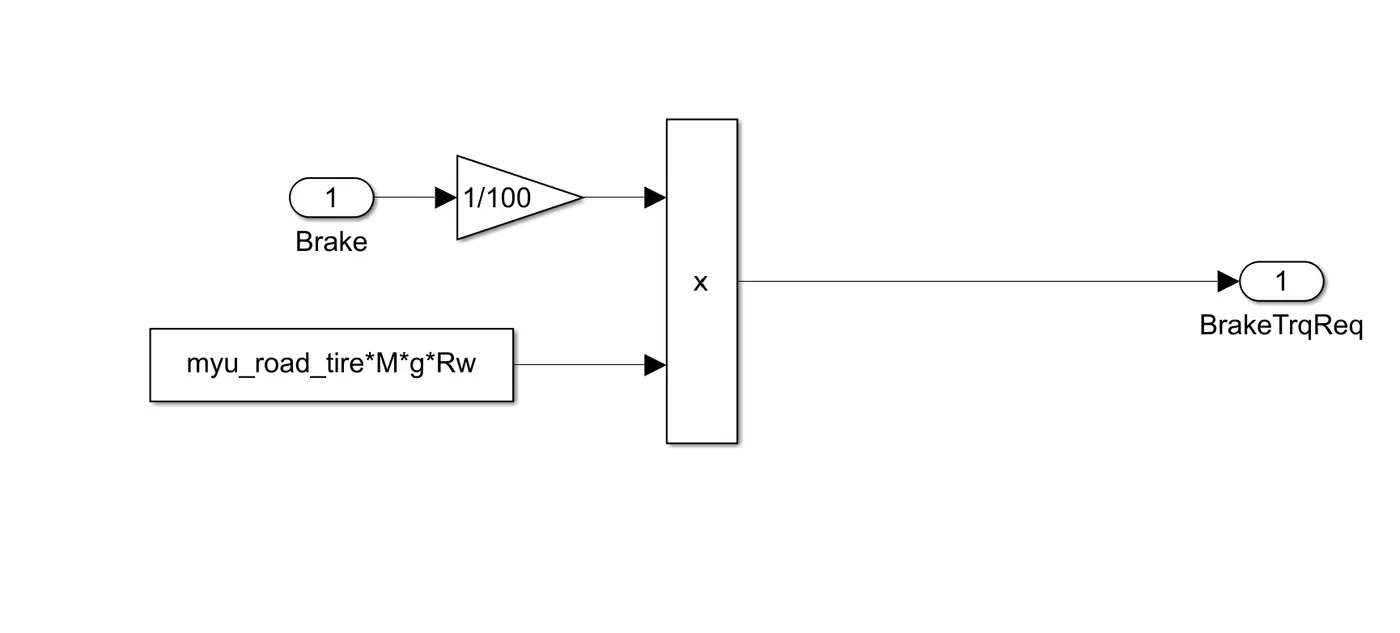
3.Brake control unit:

3.Power Train:
The powertrain encompasses every component that converts the engine's power into movement. This includes the engine, transmission, the driveshaft, differentials, axles; basically anything from the engine through to the rotating wheels.

1.Engine: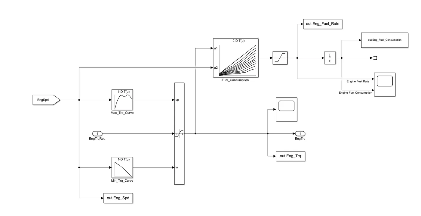

In this model we used map based model to model the fuel consumption of engine. It is based on maximum Torque and minimum torque from the controller. and then it saturated torque and give output then saturated torque and speed map give fuel consumption takes the speed and torque then the output goes into saturated then its integrated.

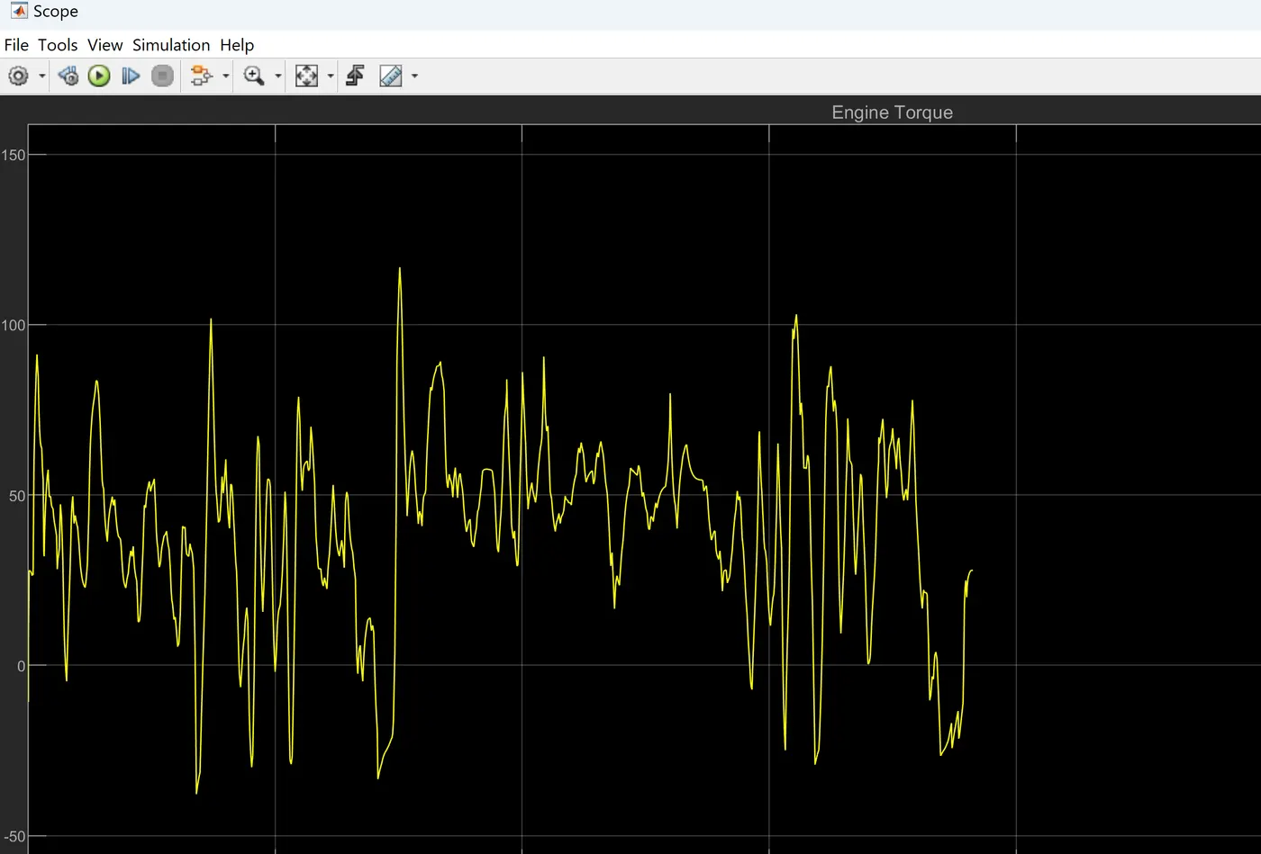
Graph:

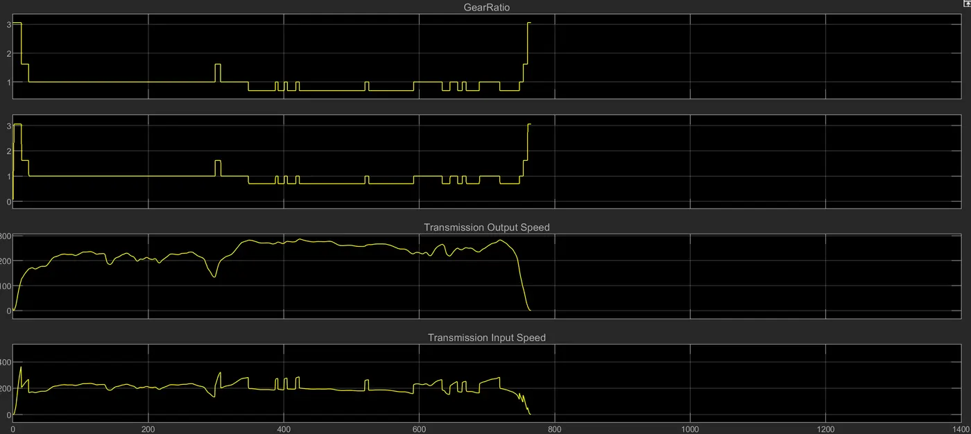
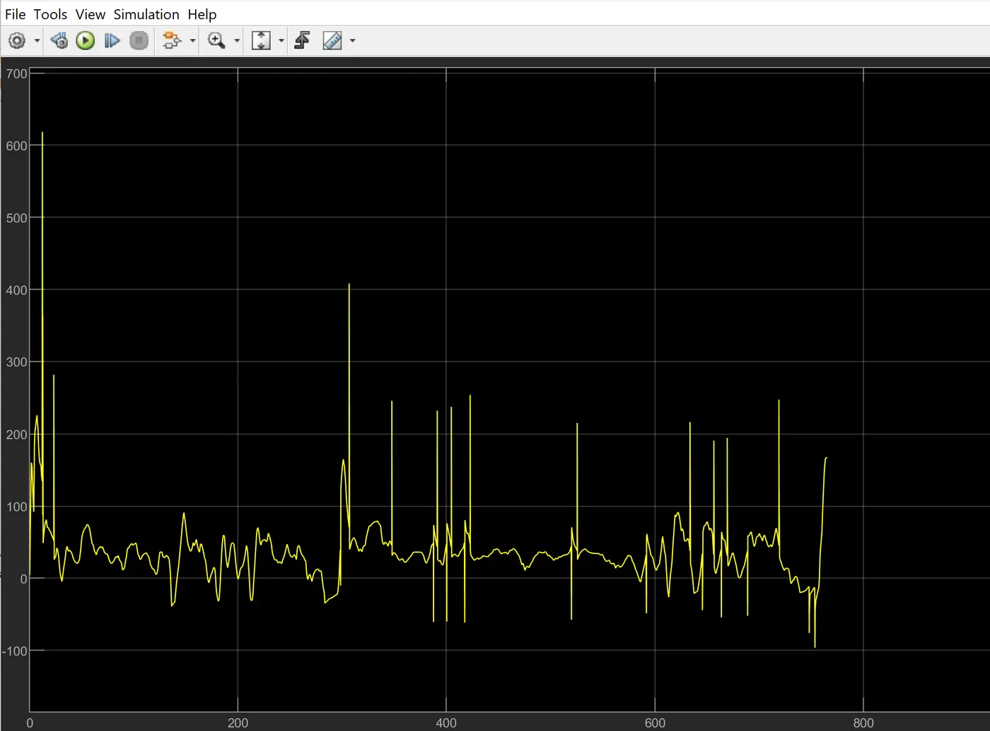
2.Transmission: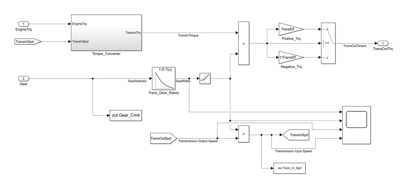

In these model we take engine torque, gear selector from controllerb for transmission of gear ratio. The ratio is multiply by transmission input torque and then the transmission efficiency positive torque and negative torque gives transmission input speed. In this case torque converter connects the engine to transmission it is part of transmission. In it basically engine dynamics and that is decoupled.

The transmission (also called the gearbox) is a part of the powertrain system that adjusts the power output from the engine or electric motor to match the required drive conditions — such as acceleration, cruising, or climbing.

Graph:

3.Differential:
In this taking input is the transmission output then its going to the differential ratio multiplied the output and input torque then meet axle torque. The axle torque is a lower than the transmission torque and differential ratio.The differential is essential for turning, handling, and power distribution.Without it, vehicles would lose traction or control, especially during cornering.Modern vehicles use advanced differentials for performance, safety, and off-road capability.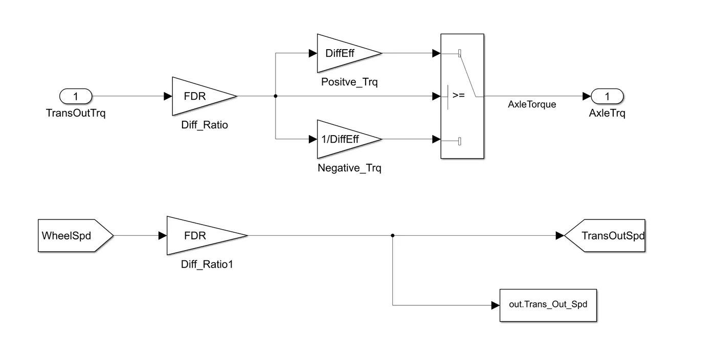

4.Wheels: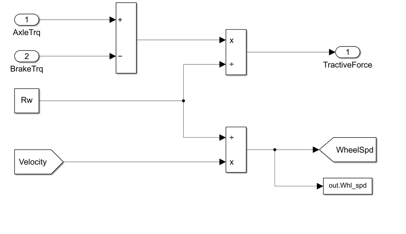

In this model we take the axle torque from differentail and brake torque from controller. it is substracts and multiplied rolling radius and velocity then we meet the tractive force from axle and brake torque. and the wheelspeed is meet using velocity.

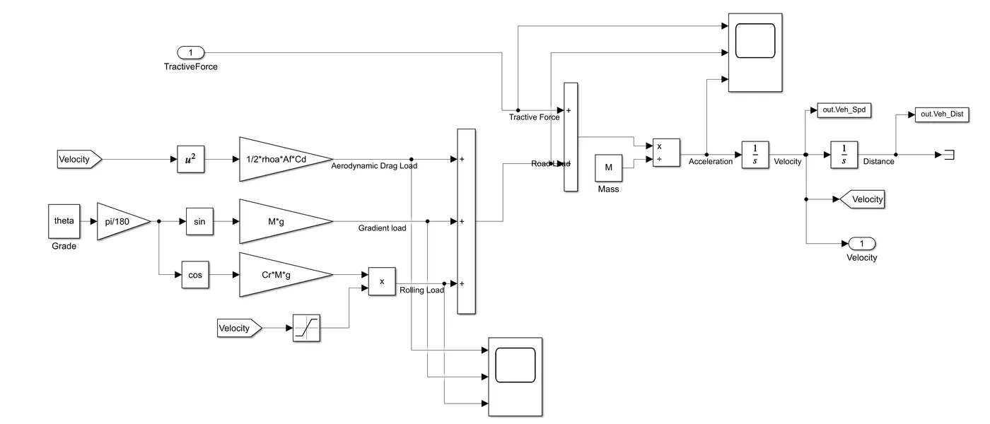
5.Vehicle dynamics:

Detailed Road Load and Tractive Effort Equation

$$M \cdot \frac{dV_{\text{veh}}}{dt} = \eta_t \cdot \lambda_{\text{tot}} \cdot \frac{R_w \cdot T_m}{r} - \left( \frac{1}{2} \cdot \rho \cdot A \cdot C_d \cdot (V_{\text{veh}} + V_{\text{wind}})^2 + C_r \cdot M \cdot g \cdot \cos(\theta) + M \cdot g \cdot \sin(\theta) \right)$$M⋅dtdVveh​​=ηt​⋅λtot​⋅rRw​⋅Tm​​−(21​⋅ρ⋅A⋅Cd​⋅(Vveh​+Vwind​)2+Cr​⋅M⋅g⋅cos(θ)+M⋅g⋅sin(θ))

---

Where:

• $M$M: Mass of the vehicle (kg)

• $\frac{dV_{\text{veh}}}{dt}$dtdVveh​​: Vehicle acceleration (m/s²)

• $\eta_t$ηt​: Transmission efficiency (dimensionless, typically 0.85–0.95)

• $\lambda_{\text{tot}}$λtot​: Overall gear ratio (dimensionless)

• $R_w$Rw​: Wheel radius (m)

• $T_m$Tm​: Motor torque (Nm)

• $r$r: Final drive ratio (if not merged with $\lambda_{\text{tot}}$λtot​)

• $\rho$ρ: Air density (kg/m³)

• $A$A: Frontal area of the vehicle (m²)

• $C_d$Cd​: Aerodynamic drag coefficient (dimensionless)

• $V_{\text{veh}}$Vveh​: Vehicle speed (m/s)

• $V_{\text{wind}}$Vwind​: Headwind speed (positive for opposing wind, m/s)

• $C_r$Cr​: Coefficient of rolling resistance (dimensionless)

• $g$g: Acceleration due to gravity (9.81 m/s²)

• $\theta$θ: Road incline angle (radians)

---

Interpretation:

• Left side: Represents the inertial force required to accelerate the vehicle.

• First term on the right: Represents the effective tractive force delivered to the wheels.

• Bracketed terms: Represent total resistive forces (aerodynamic drag, rolling resistance, and hill climb resistance).

This equation is useful for forward vehicle simulations, powertrain sizing, and energy consumption analysis.

Now for the graphs we will run the matlab code.

%%%%%%%%%%%%%%%%%%%%%%%%%%%%%%%%%%%%%%%%%%%%%%%%%%%%%%%%%%%%%%%%%%%%%

%% Skill-Lync -> Hybrid Drives Development

% Project 1 - Conventional Vehicle Model

% By - Ullekh Gambhira

% Description:

% The following file is to used with the Initialization file and Simulink

% results for post-processing of the data.

% The file is incomplete, has some examples of how the data is imported

% into a readable format, data analysis and plotting examples.

% Based on the project task, use commands in a similar format as given

% below, to analyse the data and generate required plots.

% You can change variable names if desired

%% Post-Processing File

% File for post-processing the Conventional vehicle simulation model data

%% Renaming variables

Time = out.tout;

Acc_Pdl = out.Acc_Pdl; % Accelerator pedal [%]

Brk_Pdl = out.Brk_Pdl; % Brake pedal [%]

Gear_Cmd = out.Gear_Cmd; % Transmission gear

Trans_In_Spd = out.Trans_In_Spd*30/pi; % Transmission input speed [rpm]

Trans_Out_Spd = out.Trans_Out_Spd*30/pi;% Transmission output speed [rpm]

Eng_Trq = out.Eng_Trq; % Engine brake torque [Nm]

Eng_Spd = out.Eng_Spd*30/pi; % Engine speed [rpm]

Eng_Fuel_rate = out.Eng_Fuel_Rate; % Engine Fuel Rate [g\kW]

Eng_Fuel_Consump = out.Eng_Fuel_Consumption; % Engine fuel consumption [g]

Veh_Dist = out.Veh_Dist/1000; % Distance traveled by vehicle [km]

Veh_Spd = out.Veh_Spd*18/5; % Vehicle speed [kmph]

Whl_Spd = out.Whl_spd*30/pi; % Wheel speed [rpm]

Desired_spd = out.Desired_Velo*18/5; % Desired Speed [Kmph]

%% Data Analysis

Eng_Pwr = Eng_Spd*pi/30.*Eng_Trq/1000; % Engine brake power [kW]

rho_petrol = 0.7197; % Density of petrol [kg/L]

kmpl = Veh_Dist(end)/(Eng_Fuel_Consump(end)/1000/rho_petrol); % Fuel economy [kmpl]

% Display Fuel Economy of the Cycle

fprintf('\nFuel Economy = %2.2fKmpl\n\n',kmpl);

%% Plotting vehicle characteristics time trace

% Plotting transmission input, transmission output and wheel speed

figure(1)

hold on

grid on

plot(Time, Trans_In_Spd, 'linewidth', 1, 'Color', 'black');

plot(Time, Trans_Out_Spd, 'linewidth', 1, 'Color', 'red');

plot(Time, Whl_Spd, 'linewidth', 1, 'Color', 'blue');

xlabel('Time [s]')

ylabel('Speed [rpm]')

xlim([0, Time(end)]);

legend('Trans Input','Trans Output','Wheel Speed');

% Plotting engine torque, engine power, fuel rate and fuel consumption

figure(2)

subplot(4,1,1)

hold on

grid on

plot(Time, Eng_Trq, 'linewidth', 1, 'Color', 'black');

ylabel('Torque [Nm]')

xlim([0, Time(end)]);

subplot(4,1,2)

hold on

grid on

plot(Time, Eng_Pwr, 'linewidth', 1, 'Color', 'black');

ylabel('Power [KW]')

xlim([0, Time(end)]);

subplot(4,1,3)

hold on

grid on

plot(Time, Eng_Fuel_rate, 'linewidth', 1, 'Color', 'black');

xlim([0, Time(end)]);

xlabel('Time [s]');

ylabel('Engine Fuel rate');

subplot(4,1,4)

hold on

grid on

plot(Time, Eng_Fuel_Consump, 'linewidth', 1, 'Color', 'black');

xlim([0, Time(end)]);

xlabel('Time [s]');

ylabel('Fuel Consumption [g]');

%Plotting accelerator and brake pedal gear command, vehicle desired and actual speed, vehicle distance

figure(3)

subplot(4,1,1)

hold on

grid on

plot(Time, Acc_Pdl, 'linewidth', 1, 'Color', 'black');

plot(Time, Brk_Pdl, 'linewidth', 1, 'Color', 'red');

ylabel('Pedal [%]')

xlim([0, Time(end)]);

legend('Accel','Brake');

subplot(4,1,2)

hold on

grid on

plot(Time, Gear_Cmd, 'linewidth', 1, 'Color', 'black');

xlim([0, Time(end)]);

xlabel('Time [s]');

ylabel('Gear');

subplot(4,1,3)

hold on

grid on

plot(Time, Veh_Spd, 'linewidth', 1, 'Color', 'red');

plot(Time, Desired_spd, 'linewidth', 1, 'Color', 'black');

ylabel('Speed [Kmph]')

xlim([0, Time(end)]);

legend('Actual speed','Desired speed');

subplot(4,1,4)

hold on

grid on

plot(Time, Veh_Dist, 'linewidth', 1, 'Color', 'black');

xlim([0, Time(end)]);

xlabel('Time [s]');

ylabel('Distance [Km]');

%% Plotting Drive Cycle

figure(4)

hold on

grid on

plot(cyc_time, cyc_vel, 'linewidth', 1, 'Color', 'black');

xlabel('Time [s]')

ylabel('Velocity [Mph]')

title('Drive Cycle')

% Test Results

Avg_speed = sum(Veh_Spd)/length(Veh_Spd);

Max_Speed = maxk(Veh_Spd,1);

table(Avg_speed,Max_Speed,kmpl,'VariableNames',{'Average Speed [kmph]','Maximum Speed [kmph]','Fuel Economy [kmpl]'})

%% Plotting engine operating points on engine fuel map

figure('Name','Engine Operating Points');

hold on

grid on

title('Engine Operating Points','fontsize',12);

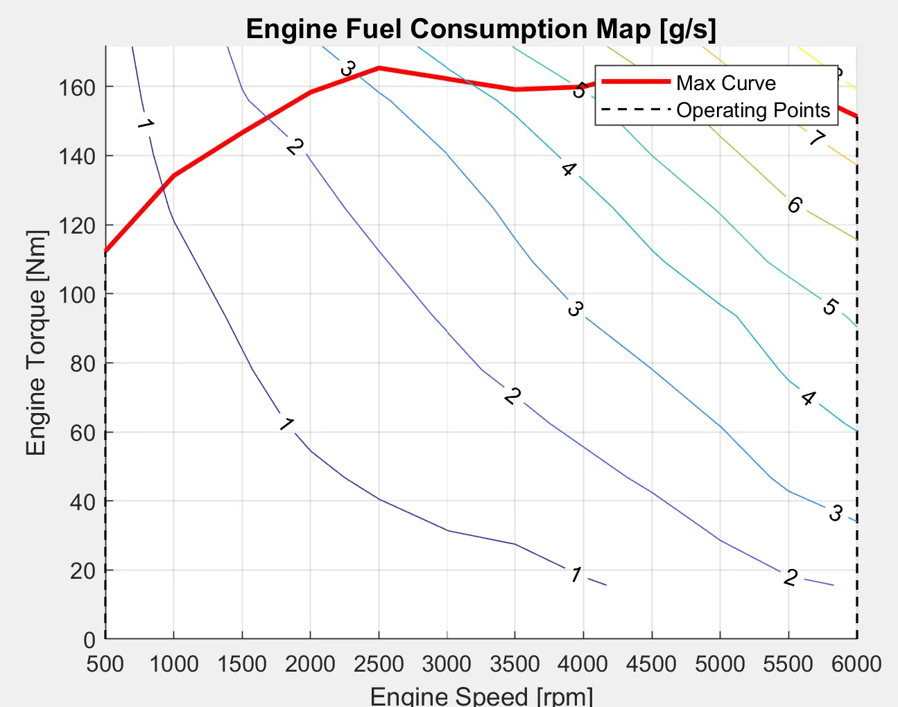
p1=plot(Eng_map_spd*30/pi,Eng_max_trq,'linewidth',2,'color','r');

p2=line([Eng_map_spd(end)*30/pi Eng_map_spd(end)*30/pi],[0 Eng_max_trq(end)]);

set(p2,'linewidth',1,'linestyle','--','color','k');

p3=line([Eng_map_spd(1)*30/pi Eng_map_spd(1)*30/pi],[0 Eng_max_trq(1)]);

set(p3,'linewidth',1,'linestyle','--','color','k');

[c,h] = contour(Eng_map_spd'*30/pi,Eng_map_trq,Eng_fuel_map');

clabel(c,h);

xlabel('Engine Speed [rpm]');

ylabel('Engine Torque [Nm]');

title('Engine Fuel Consumption Map [g/s]');

legend({'Max Curve','Operating Points'});

axis([Eng_map_spd(1)*30/pi Eng_map_spd(end)*30/pi 0 Eng_map_trq(end)]);

1.Plotting transmission input, transmission output and wheel speed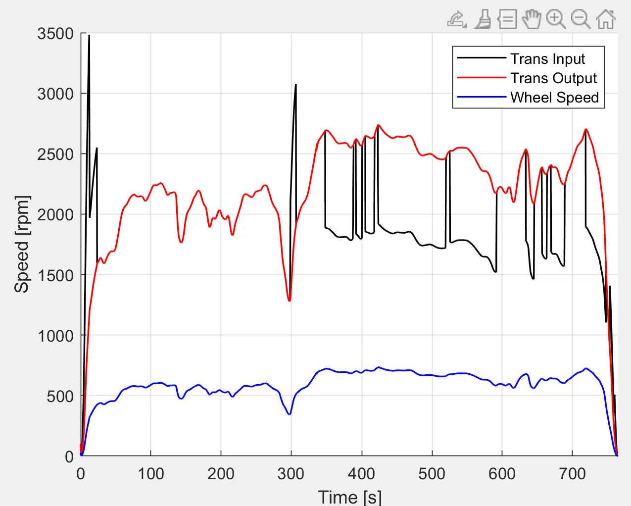

In this graph we see the transmission input and transmission out will fluctuates up and down as increasing speed and time.

2.Plotting engine torque, engine power, fuel rate and fuel consumption: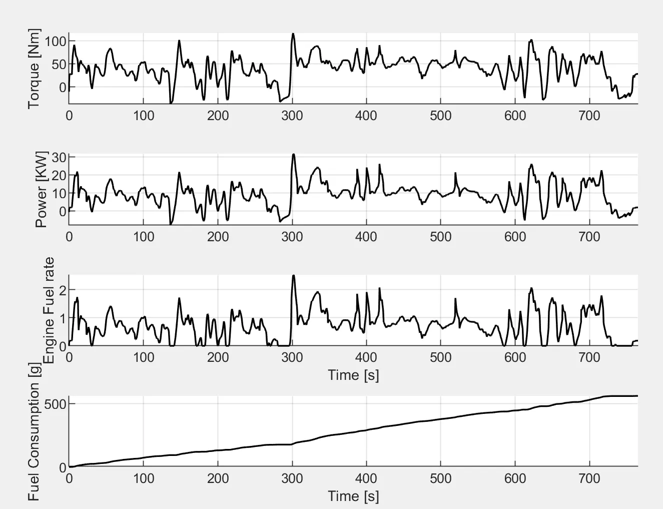

3.Plotting accelerator and brake pedal gear command, vehicle desired and actual speed, vehicle distance: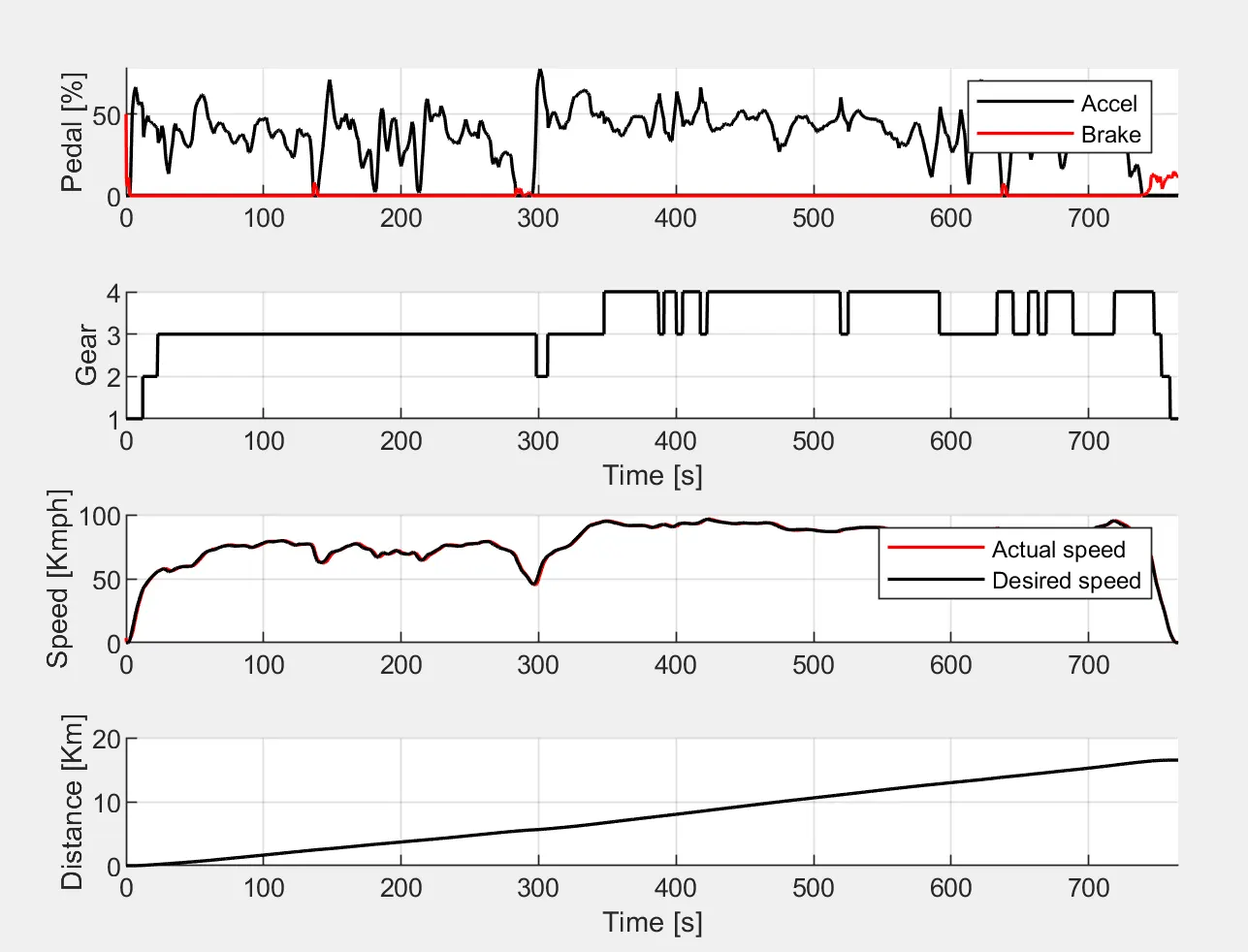

4.Plotting Drive Cycle: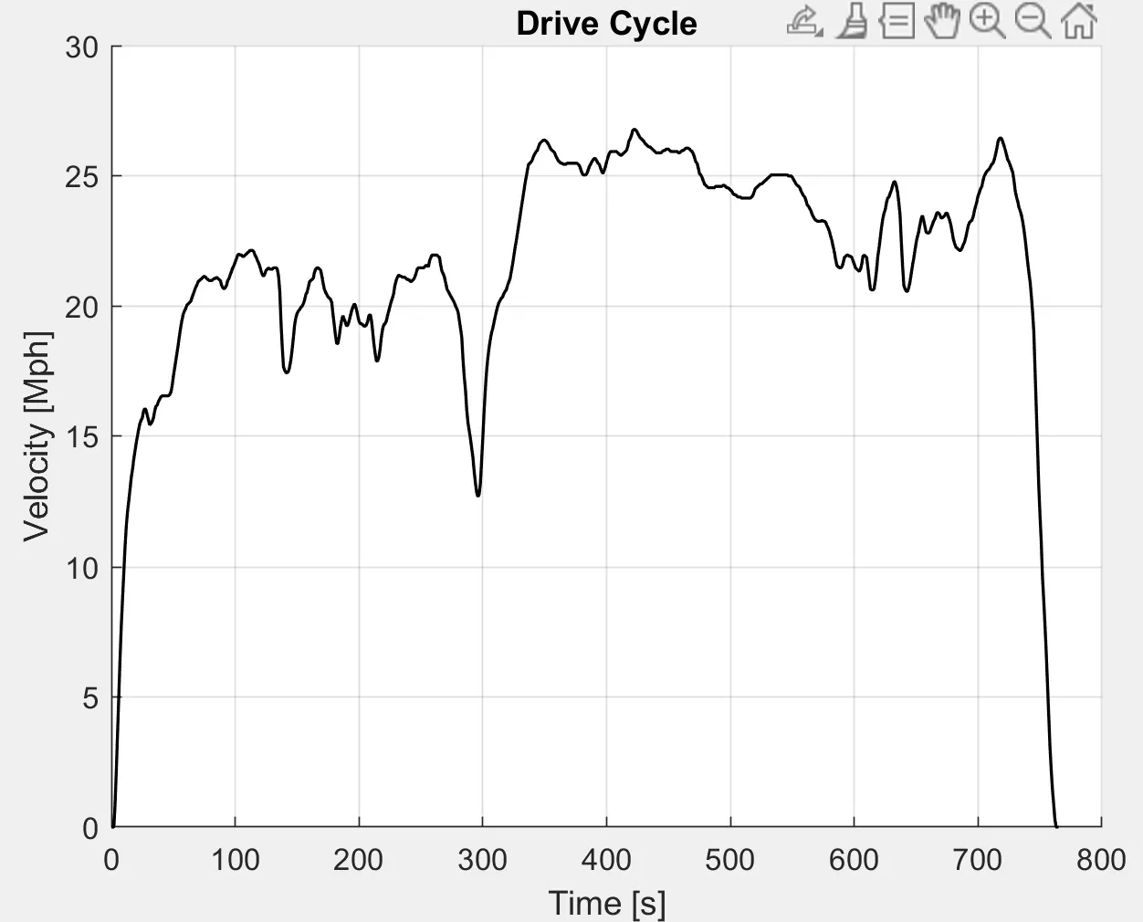

5.Plotting engine operating points on engine fuel map: