Project 1
Aim :- To develop a forward energy-based fuel consumption model of a conventional vehicle and plot the required parameters using given data for UDDS drive cycle and HWFET drive cycle.
Theory :- Forward Models are a dynamic simulation which are used for detailed simulations. Force, Torque or power are the inputs and vehicle state variables like velocity, acceleration are outputs. And there is also a feedback loop to meet desired vehicle state. The following figure shows the Forward Model of a vehicle with actual speed feedback.
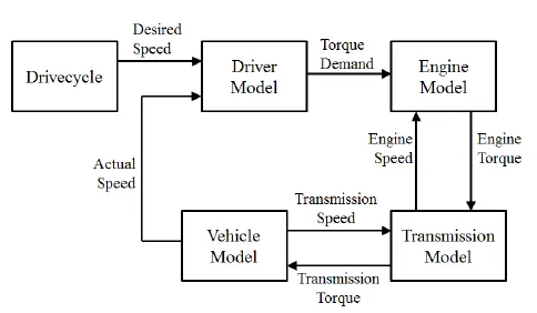
Drive Cycle is a series of data points representing the speed of a vehicle versus time. Driving cycles are produced by different countries and organizations to assess the performance of vehicles in various ways, as for instance fuel consumption, electric vehicle autonomy and polluting emissions. In this simulation the drive cycles such as UDDS( Urban Dynamometer Driving Schedule) and HWFET (The Highway Fuel Economy Test) are analysed for a conventional forward model of a vehicle. For more information on drive cycles :- Ref link given in end
Procedure :- The simulation is carried out in 3 stages. In first stage all the variables required for the simulink model are loaded in matlab workspace, in second stage the vehicle model is developed in simulink environment and send the required values to matlab workspace, and in final stage the postprocessing is done by using simulink values that sent to matlab workspace. By using this values, The graphs are generated.
Stage 1 Initialization
1. Open given matlab initialisation file. This file consists of the required variables, conversions from m/s to kmph, and all other necessary manipulations are shown in code as comments.
2. Run the script to get required variables.
3. Change the drive cycle values. They are assigned to numbers from 1 to 6 using else if conditions. For UDDS type 1 and for HWFET type 2 in Drive_Cycle_Select.
Code:-
%%%%%%%%%%%%%%%%%%%%%%%%%%%%%%%%%%%%%%%%%%%%%%%%%%%%%%%%%%%%%%%%%%%%%
%% Skill-Lync -> Hybrid Drives Development
% Project 2 - P1 Hybrid Vehicle Model
% By - Aditya Kurup

% Description:

%% Initialization File
% Initialization file for loading the variables for the Conventional vehicle simulation model

%% Vehicle Parameters
M = 1500;       % Vehicle weight [kg]
Cr = 0.015;     % Rolling resistance coefficient
Rw = 0.35;      % Rolling radius [m]
Cd = 0.33;      % Drag coefficient
Af = 2;         % Frontal area [m2]
rhoa = 1.225;   % Air density [kg/m3]
Vwind = 0;      % Wind velocity [kmph]
g = 9.81;       % Gravitational acceleration [m/s2]
theta = 0;      % Slope [deg]
myu_road_tire = 1; % Coefficient of friction between tire - road interface

%% Powertrain Parameters
FDR = 3.73;                         % Final Drive Ratio / Diff Ratio
DiffEff = 0.99;                     % Differential efficiency (assumed independent of operating conditions)

NumGear = 4;                        % Number of gears in transmission
TransGear = [1:NumGear];            % Transmission Gears
TransRatio = [3.06, 1.62, 1, 0.7];  % Corresponding Transmission ratios
TransEff = 0.90;                    % Transmission efficiency (assumed independent of operating conditions)

TC_SR = [0, .5, .6, .7, .8, .87, .92, .94, .96, .97, 1];   % Torque Converter Speed Ratio (Matlab default) -> TurbSpd/PumpSpd
TC_TR = [2.232, 1.5462, 1.4058, 1.2746, 1.1528, 1.0732, 1.0192, 1, 1, 1, 1];   % Torque Converter Torque Ratio (Matlab default) -> TurbTrq/PumpTrq
TC_Cf = 1e-4 * [.72558, .66322, .63463, .59042, .51331, .4144, .29287, .22444, .12186, .04386, 0]; % Torque Converter Capacity Factor (Matlab default) -> PumpTrq/PumpSpd^2 [Nm/rpm^2]

load Vehicle_Data/Engine_data_1_9L_Saturn_95kW
load Vehicle_Data/Trans_Shift_map
load Vehicle_Data/EM_Honda_Insight_10kW
load Vehicle_Data/ESS_NiMH6


ESS_init_soc = 0.8;
ESS_soc_max = 0.9;
ESS_soc_min = 0.6;


%% Driver Parameters
Kp = 10;                    % P gain for driver PI model
Ki = 1;                     % I gain for driver PI model
Drive_Cycle_Select = 1;     % Drive cycle selection

%% Inputting the desired DriveCycle
%Drive_Cycle_Select = input(sprintf('Select a Drive Cycle: n 1. UDDS n 2. HWFET n 3. FTP n 4. US06 n 5. NEDC n 6. WLTP n Your selection is: '));
% Drive cycle values in m/s

%Loading Drive Cycle values. Variables: cyc_time, cyc_vel
if Drive_Cycle_Select == 1
    load DriveCycles/UDDS;

elseif Drive_Cycle_Select == 2
    load DriveCycles/HWFET;

elseif Drive_Cycle_Select == 3
    load DriveCycles/FTP;

elseif Drive_Cycle_Select == 4
    load DriveCycles/US06;

elseif Drive_Cycle_Select == 5
    load DriveCycles/NEDC;

elseif Drive_Cycle_Select == 6
    load DriveCycles/WLTP;

end

time_end = cyc_time(end); %Drive cycle end time
vel_end = cyc_vel(end); %Drive cycle end velocity

%% Running Simulink Model
%sim('Project2_VehicleModel');   % Run Simulink model
Stage 2 Developing a model in simulink for the forward fuel consumption model of a vehicle.
- The main simulink model is shown below. It has Driver, Controller and Power train as shown
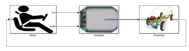
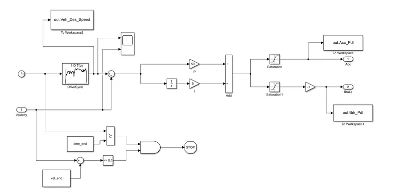
A. Driver :- All the inputs to vehicle like acceleration and braking are given through this block. This block is responsible for implementing the required drive cycle. The inputs like velocity follows the drive cycle and the velocity is controlled by braking. The PI is a feedback control loop that calculates an error signal by taking the difference between the output of a system, in this case the signal is velocity.
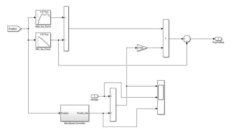
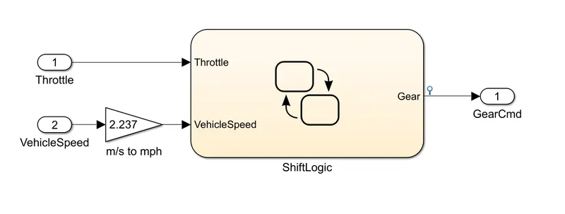
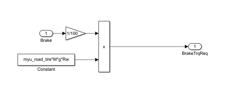
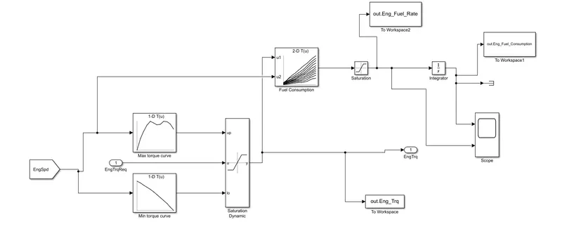
B. Controller :- The Controller block is the brains of the vehicle, representing the electronic controls units. Based on the driver inputs, it generates desired engine torque, desired transmission gear and desired brake torque. These inputs are fed to the Powertrain block. The controller has 3 sub blocks which are Engine Control unit, Transmssion control unit and Brake control unit. The maximum and minimum torque curves are feed into lookup table.
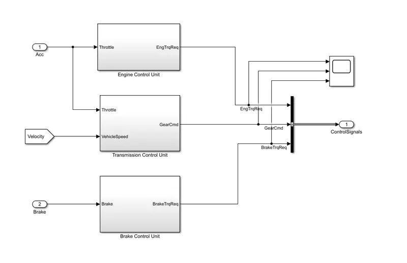
ENGINE CONTROL UNIT :-
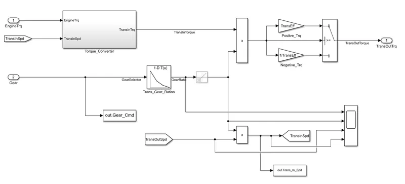
TRANSMISSION CONTROL UNIT:-
BRAKE CONTROL UNIT :-
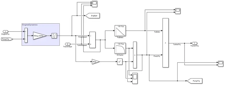
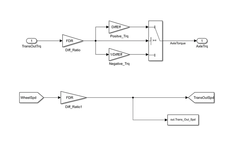
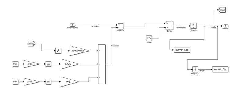
C. Power Train :- Powertrain block represents the drivetrain of the vehicle. It consists of an Engine connected to the Automatic Transmission through a Torque Converter’. The output of the transmission is connected to the Differential, which powers the Wheels, that provides the tractive force for vehicle acceleration. The longitudinal dynamics of the vehicle along with the road load is represented in the Vehicle Dynamics block.
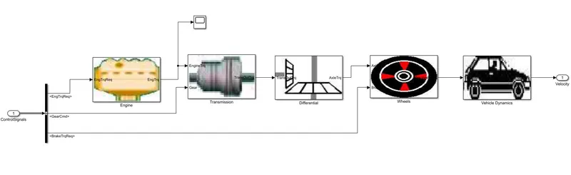
ENGINE :-
TRANSMISSION :-
TORQUE CONVERTER :-
DIFFERENTIAL :-
WHEELS :-
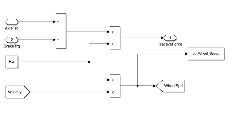
VEHICLE DYNAMICS :- This block is modeled by referencing the below formula.

Stage 3 Post Processing the results
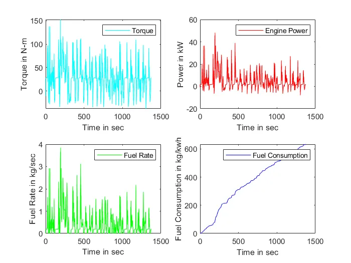
The graphs are drawn from the data from simulink. The required data from required systems is sent to matlab using 'To wokspace' block. The output data is changed to Array from Time series. The code for conversions, calculation of kmpl and plotting the graphs are shown below.
%% Renaming variables
Time = out.tout;
Acc_Pdl = out.Acc_Pdl;          % Accelerator pedal [%]
Brk_Pdl = out.Brk_Pdl;          % Brake pedal [%]
Gear_Cmd = out.Gear_Cmd;        % Transmission gear
Trans_In_Spd = out.Trans_In_Spd*30/pi;  % Transmission input speed [rpm]
Trans_Out_Spd = out.Trans_Out_Spd*30/pi;% Transmission output speed [rpm]
Eng_Trq = out.Eng_Trq;          % Engine brake torque [Nm]
Eng_Spd = out.Eng_Spd*30/pi;    % Engine speed [rpm]
Eng_Fuel_Consump = out.Eng_Fuel_Consumption;    % Engine fuel consumption [g]
Eng_Fuel_Rate = out.Eng_Fuel_Rate;   %Engine fuel rate in Kg/sec
Veh_Dist = out.Veh_Dist/1000;   % Distance traveled by vehicle [km]
Veh_Spd = out.Veh_Spd*18/5;     % Vehicle speed [kmph]
Wheel_Speed = out.Wheel_Speed;  %Wheel speed [rad/sec]
Vehicle_Desired_Speed = out.Veh_Des_Speed*18/5;  %Vehicle desired speed from drive cycle in kmph


% Data Analysis
Eng_Pwr = Eng_Spd.*pi/30.*Eng_Trq/1000;   % Engine brake power [kW]
rho_petrol = 0.7197;                    % Density of petrol [kg/L]
kmpl = Veh_Dist(end)/(Eng_Fuel_Consump(end)/1000/rho_petrol);    % Fuel economy [kmpl]

%%Plotting Graphs

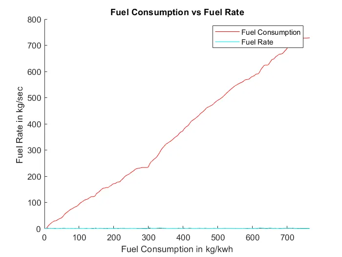
% Plotting Fuel Consumption vs Fuel Rate
figure(1)
hold on
plot(Time, Eng_Fuel_Consump, 'Color', 'r');
plot(Time, Eng_Fuel_Rate,'Color', 'c');
title('Fuel Consumption vs Fuel Rate')
xlabel('Fuel Consumption in kg/kwh')
ylabel('Fuel Rate in kg/sec ')
xlim([0, Time(end)]);
legend('Fuel Consumption','Fuel Rate');


%Plotting vehicle characteristics time trace Engine,Transmission Input, Transmission Output and Wheel Speed
figure(2)
hold on
plot(Time,Eng_Spd,'color','k');
plot(Time,Trans_In_Spd,'color','b');
plot(Time,Trans_Out_Spd,'color','g');
plot(Time,Wheel_Speed,'color','r');
xlabel('Time in s')
ylabel('Speed in rpm')
xlim([0, Time(end)]);
ylim([0, 6000]);
legend('Engine Speed','Transmission Input','Transmission Output','Wheel Speed');

% Plotting vehicle characteristics time trace engine torque, engine power,
% fuel rate and fuel consumption.
figure(3)
subplot(2,2,1)
plot(Time,Eng_Trq,'color','c')
xlabel('Time in sec')
ylabel('Torque in N-m')
legend('Torque')

subplot(2,2,2)
plot(Time,Eng_Pwr,'Color','r')
xlabel('Time in sec')
ylabel('Power in kW')
legend('Engine Power')

subplot(2,2,3)
plot(Time,Eng_Fuel_Rate,'color','g')
xlabel('Time in sec')
ylabel('Fuel Rate in kg/sec')
legend('Fuel Rate')

subplot(2,2,4)
plot(Time,Eng_Fuel_Consump,'color','b')
xlabel('Time in sec')
ylabel('Fuel Consumption in kg/kwh')
legend('Fuel Consumption')


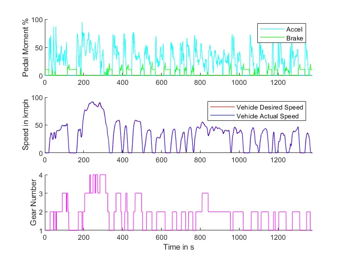
%Plotting accelerator and brake pedal, gear command, vehicle desired and
%actual speed, vehicle distance.
figure(4)
subplot(3,1,1)
hold on
plot(Time, Acc_Pdl, 'color', 'c');
plot(Time, Brk_Pdl, 'color', 'g');
ylabel('Pedal Moment %')
xlim([0, Time(end)]);
legend('Accel','Brake');

subplot(3,1,2)
hold on
plot(Time,Vehicle_Desired_Speed.Data, 'color', 'r');
plot(Time,Veh_Spd.Data, 'color', 'b');
ylabel('Speed in kmph')
xlim([0, Time(end)]);
legend('Vehicle Desired Speed','Vehicle Actual Speed');


subplot(3,1,3)
hold on
plot(Time, Gear_Cmd, 'color', 'm');
xlim([0, Time(end)]);
xlabel('Time in s');
ylabel('Gear Number');

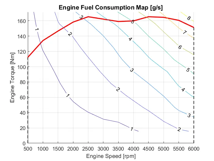
%% Plotting engine operating points on engine fuel map
figure('Name','Engine Operating Points');
hold on
grid on
title('Engine Operating Points','fontsize',12);
p1=plot(Eng_map_spd*30/pi,Eng_max_trq,'linewidth',2,'color','r');
p2=line([Eng_map_spd(end)*30/pi Eng_map_spd(end)*30/pi],[0 Eng_max_trq(end)]);
set(p2,'linewidth',1,'linestyle','--','color','k');
p3=line([Eng_map_spd(1)*30/pi Eng_map_spd(1)*30/pi],[0 Eng_max_trq(1)]);
set(p3,'linewidth',1,'linestyle','--','color','k');
[c,h] = contour(Eng_map_spd'*30/pi,Eng_map_trq,Eng_fuel_map');
clabel(c,h);
xlabel('Engine Speed [rpm]');
ylabel('Engine Torque [Nm]');
title('Engine Fuel Consumption Map [g/s]');
%p4 = plot(Eng_Spd,Eng_Trq,'.','color','k');
%legend([p1 p4],{'Max Curve','Operating Points'});
axis([Eng_map_spd(1)*30/pi Eng_map_spd(end)*30/pi 0 Eng_map_trq(end)]);
Results and observations :-
The fuel economy (kmpl) for UDDS and HWFET are tabulated below.
| Drive Cycle | UDDS | HWFET |
| Fuel Economy in (kmpl) | 13.6312 | 16.307 |
UDDS Cycle :-
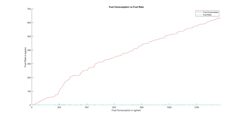
1. Fuel Consumption vs Fuel rate :-
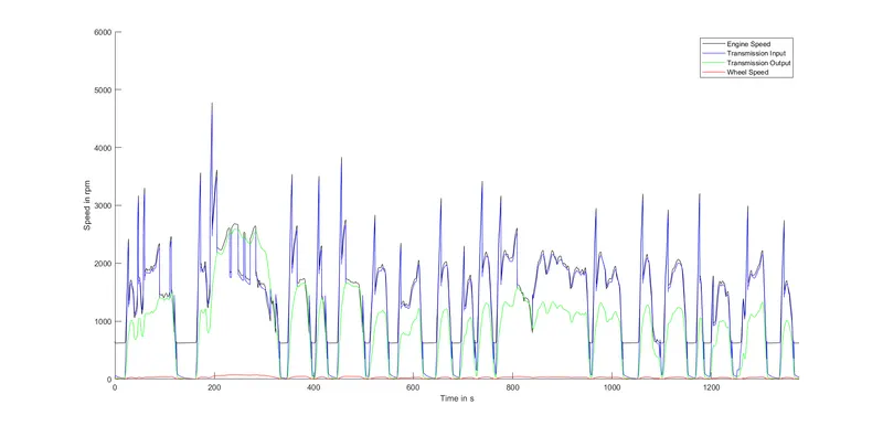
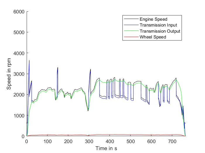
2. Time trace for engine, transmission input, transmission output and wheel speed
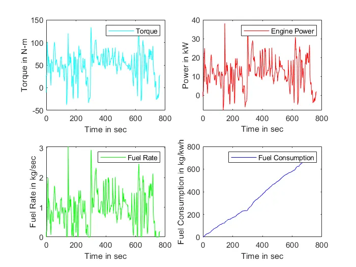
3. Engine torque, engine power, fuel rate and fuel consumption
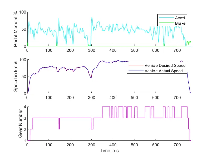
4. Accelerator and brake pedal, Gear Number, vehicle desired and actual speed
5. Engine operating points on the engine fuel map.
HWFET Cycle :-
1. Fuel Consumption vs Fuel rate :-
2. Time trace for engine, transmission input, transmission output and wheel speed
3. Engine torque, engine power, fuel rate and fuel consumption
4. Accelerator and brake pedal, Gear Number, vehicle desired and actual speed
5. Engine operating points on the engine fuel map.
By observing the above graphs from UDDS and HWFET drive cycles
1. The fuel economy is best in HWFET as HWFET is highway driving as it doesn't require much variations in driving conditions.
2. The fluctuations in UDDS are more than HWFET.
3. The more the fluctuations in speed, the change of gears must be more frequent. In the 3rd graph from both cycles, the UDDS requires shifting of gears more often.
4. From the above observations it is obvious that more frequent changes in engine operating conditions is not economical as the fuel economy will decrease.
Reference:
1. https://www.epa.gov/vehicle-and-fuel-emissions-testing/dynamometer-drive-schedules