Project 1
Ans) To compute the fuel economy numbers for the given vehicle (kmpl) on the urban cycle (UDDS)Also, to analyze and understand the vehicle operating points in terms of engine speed, torque, transmission speeds, pedal positions, gear, distance traveled, etc.
Drive Cycle -1 (UDDS)
Project-1 Initial_File.m
%%%%%%%%%%%%%%%%%%%%%%%%%%%%%%%%%%%%%%%%%%%%%%%%%%%%%%%%%%%%%%%%%%%%%
%% Skill-Lync -> Hybrid Drives Development
% Project 1 - Conventional Vehicle Model
% By - Ullekh Gambhira

% Description:

%% Initialization File
% Initialization file for loading the variables for the Conventional vehicle simulation model

%% Vehicle Parameters
M = 1500;       % Vehicle weight [kg]
Cr = 0.015;     % Rolling resistance coefficient
Rw = 0.35;      % Rolling radius [m]
Cd = 0.33;      % Drag coefficient
Af = 2;         % Frontal area [m2]
rhoa = 1.225;   % Air density [kg/m3]
Vwind = 0;      % Wind velocity [kmph]
g = 9.81;       % Gravitational acceleration [m/s2]
theta = 0;      % Slope [deg]
myu_road_tire = 1; % Coefficient of friction between tire - road interface

%% Powertrain Parameters
FDR = 3.73;                         % Final Drive Ratio / Diff Ratio
DiffEff = 0.99;                     % Differential efficiency (assumed independent of operating conditions)

NumGear = 4;                        % Number of gears in transmission
TransGear = [1:NumGear];            % Transmission Gears
TransRatio = [3.06, 1.62, 1, 0.7];  % Corresponding Transmission ratios
TransEff = 0.90;                    % Transmission efficiency (assumed independent of operating conditions)

TC_SR = [0, .5, .6, .7, .8, .87, .92, .94, .96, .97, 1];   % Torque Converter Speed Ratio (Matlab default) -> TurbSpd/PumpSpd
TC_TR = [2.232, 1.5462, 1.4058, 1.2746, 1.1528, 1.0732, 1.0192, 1, 1, 1, 1];   % Torque Converter Torque Ratio (Matlab default) -> TurbTrq/PumpTrq
TC_Cf = 1e-4 * [.72558, .66322, .63463, .59042, .51331, .4144, .29287, .22444, .12186, .04386, 0]; % Torque Converter Capacity Factor (Matlab default) -> PumpTrq/PumpSpd^2 [Nm/rpm^2]

load Vehicle_Data/Engine_data_1_9L_Saturn_95kW
load Vehicle_Data/Trans_Shift_map

%% Driver Parameters
Kp = 10;                    % P gain for driver PI model
Ki = 1;                     % I gain for driver PI model
Drive_Cycle_Select = 1;     % Drive cycle selection

% Drive cycle values in m/s

if Drive_Cycle_Select == 1
    load DriveCycles/UDDS;

elseif Drive_Cycle_Select == 2
    load DriveCycles/HWFET;

elseif Drive_Cycle_Select == 3
    load DriveCycles/FTP;

elseif Drive_Cycle_Select == 4
    load DriveCycles/US06;

elseif Drive_Cycle_Select == 5
    load DriveCycles/NEDC;

elseif Drive_Cycle_Select == 6
    load DriveCycles/WLTP;

end

time_end = cyc_time(end);
vel_end = cyc_vel(end);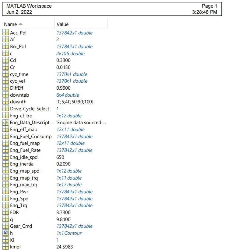
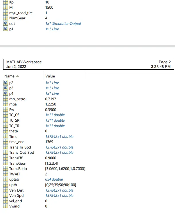
a) Vehicle Dynamics
1. constant blocks:- The Constant block produces a genuine or complex consistent worth sign. Utilize this block to give steady sign info. The block creates scalar, vector, or lattice yield, contingent upon The dimensionality of the Constant worth boundary.
Aggregate blocks:- The Sum block performs expansion or deduction on its bits of feedback. The Add, Subtract, Sum of Elements, and Sum blocks are indistinguishable blocks. This block can add or take away scalar, vector, or lattice inputs. It can likewise fall the components of a sign and play out a summation.
3. Subtract blocks
4. integrator blocks:- The Integrator block acknowledges and yields signs of type twofold on its information ports. The outside reset port acknowledges signs of type twofold or Boolean.
5. gain blocks:- The Gain block duplicates or ADD the contribution by a consistent worth (gain). The information and the increase can each be a scalar, vector, or lattice. You determine the worth of gain in the Gain boundary. The Multiplication boundary allows you to indicate component-wise or lattice increase.
6. go to and from blocks:- The Goto block passes its contribution to its relating From blocks. The information can be a genuine or complex-esteemed sign or vector of any information type. From and Goto blocks permit you to pass a sign starting with one block and then onto the next without really interfacing them.
7. trigonometry blocks:- The Trigonometric Function block carries out various normal geometrical roles. You can choose one of these capacities from the Function list: sin, cos, tan, asin, cos , tan , atan2, sinh, cosh, and tanh . The block yield is the consequence of the activity of the capacity on the info or data sources.
8. scope blocks:- The Scope block shows its contribution as for recreation time. The Scope block can have different tomahawks (one for every port); all tomahawks make some normal memories range with free y-tomahawks. The Scope permits you to change how much time and the scope of info values showed.
to work area impedes:- The To Workspace block composes input signal information to a work area. During reproduction, the block composes information for inside support. At the point when you stop the reproduction or the reenactment finishes, that information is kept in touch with the work area.
B) Engine
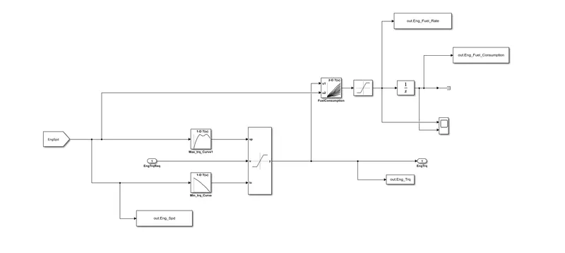
1. integrator blocks:- The Integrator block acknowledges and yields signs of type twofold on its information ports. The outside reset port acknowledges signs of type twofold or Boolean.
2. go to and from blocks:- The Goto block passes its contribution to its comparing From blocks. The info can be a genuine or complex-esteemed sign or vector of any information type. From and Goto blocks permit you to pass a sign starting with one block and then onto the next without really interfacing them.
3. to work area hinders:- The To Workspace block composes input signal information to a work area. During reproduction, the block composes information to an inside cradle. At the point when you stop the recreation or the reproduction finishes, that information is kept in touch with the work area.
4..scope blocks:- The Scope block shows its contribution regarding reenactment time. The Scope block can have numerous tomahawks (one for every port); all tomahawks make some normal memories range with autonomous y-tomahawks. The Scope permits you to change how much time and the scope of information values showed.
5.1-D Lookup table produces a result signal by introducing in view of a given informational collection and information esteem. The Input values x property should be a stringently expanding or diminishing exhibit.
2-D query table blocks:- The Lookup Table (2D) block processes a guess of result esteem with given upsides of two (2D) sources of info and results utilizing the predetermined query strategy.
7. Saturation Dynamic blocks:- The Saturation block delivers a result signal that is the worth of the info signal limited to the upper and lower immersion values. The upper and lower limits are determined by the boundaries Upper cutoff and Lower limit.
Immersion Blocks:- The Saturation block forces upper and lower limits on a sign. At the point when the info signal is inside the reach determined by as far as possible and Upper cutoff boundaries, the information signal goes through unaltered.
Project-1 Processing_File.m
%%%%%%%%%%%%%%%%%%%%%%%%%%%%%%%%%%%%%%%%%%%%%%%%%%%%%%%%%%%%%%%%%%%%%
%% Skill-Lync -> Hybrid Drives Development
% Project 1 - Conventional Vehicle Model
% By - Ullekh Gambhira

% Description:
% The following file is to used with the Initialization file and Simulink
% results for post-processing of the data.
% The file is incomplete, has some examples of how the data is imported
% into a readable format, data analysis and plotting examples.
% Based on the project task, use commands in a similar format as given
% below, to analyse the data and generate required plots.
% You can change variable names if desired

%% Post-Processing File
%  File for post-processing the Conventional vehicle simulation model data

%% Renaming variables
Time = out.tout;
Acc_Pdl = out.Acc_Pdl;          % Accelerator pedal [%]
Brk_Pdl = out.Brk_Pdl;          % Brake pedal [%]
Gear_Cmd = out.Gear_Cmd;        % Transmission gear
Trans_In_Spd = out.Trans_In_Spd*30/pi;  % Transmission input speed [rpm]
Trans_Out_Spd = out.Trans_Out_Spd*30/pi;% Transmission output speed [rpm]
Eng_Trq = out.Eng_Trq;          % Engine brake torque [Nm]
Eng_Spd = out.Eng_Spd.*30/pi;    % Engine speed [rpm]
Eng_Fuel_Consump = out.Eng_Fuel_Consumption;    % Engine fuel consumption [g]
Veh_Dist = out.Veh_Dist/1000;   % Distance traveled by vehicle [km]
Veh_Spd = out.Veh_Spd*18/5;     % Vehicle speed [kmph]
Eng_Fuel_Rate = out.Eng_Fuel_Rate;%Engine Fuel rate

%% Data Analysis
Eng_Pwr = Eng_Spd*pi/30.*Eng_Trq/1000;   % Engine brake power [kW]
rho_petrol = 0.7197;                    % Density of petrol [kg/L]
kmpl = Veh_Dist(end)/(Eng_Fuel_Consump(end)/1000/rho_petrol);    % Fuel economy [kmpl]


%% Plotting vehicle characteristics time trace
figure(1)
subplot(3,1,1)
hold on
grid on
plot(Time,Eng_Spd, 'linewidth', 1, 'Color', 'black');
ylabel('Eng_Spd')
xlim([0, Time(end)]);
legend('Eng_Spd');
subplot(3,1,2)
hold on
grid on
plot(Time, Trans_In_Spd, 'linewidth', 1, 'Color', 'black');
plot(Time, Trans_Out_Spd, 'linewidth', 1, 'Color', 'red');
ylabel('Speed [rpm]')
xlim([0, Time(end)]);
ylim([0, 6000]);
legend('Trans Input','Trans Output');
subplot(3,1,3)
hold on
grid on
plot(Time,Veh_Spd, 'linewidth', 1, 'Color', 'blue');
xlim([0, Time(end)]);
xlabel('Time [s]');
ylabel('Veh_Spd');
legend('veh_Spd');

figure(2)
subplot(3,1,1)
hold on
grid on
plot(Time,Eng_Trq, 'linewidth', 1, 'Color', 'black');
ylabel('Eng_Trq')
xlim([0, Time(end)]);
legend('Eng_Trq');
subplot(3,1,2)
hold on
grid on
plot(Time, Eng_Pwr , 'linewidth', 1, 'Color', 'red');
ylabel('Eng_Pwr]')
xlim([0, Time(end)]);
legend('Eng_Pwr');
subplot(3,1,3)
hold on
grid on
plot(Time,Eng_Fuel_Consump, 'linewidth', 1, 'Color', 'blue');
xlim([0, Time(end)]);
xlabel('Time [s]');
ylabel('Eng_Fuel_Consump');
legend('Eng_Fuel_Consump');

figure(3)
subplot(3,1,1)
hold on
grid on
plot(Time,Eng_Trq, 'linewidth', 1, 'Color', 'black');

ylabel('Eng_Trq')
xlim([0, Time(end)]);
legend('Eng_Trq');
subplot(3,1,2)
hold on
grid on
plot(Time, Eng_Pwr , 'linewidth', 1, 'Color', 'green');
ylabel('Eng_Pwr]')
xlim([0, Time(end)]);
legend('Eng_Pwr');
subplot(3,1,3)
hold on
grid on
plot(Time,Eng_Fuel_Rate , 'linewidth', 1, 'Color', 'red');
xlim([0, Time(end)]);
xlabel('Time [s]');
ylabel('Eng_Fuel_Rate ');
legend('Eng_Fuel_Rate ');

figure(4)
subplot(4,1,1)
hold on
grid on
plot(Time,Acc_Pdl, 'linewidth', 1, 'Color', 'black');
plot(Time, Brk_Pdl, 'linewidth', 1, 'Color', 'red');
ylabel('Acc_Pdl & Brk_Pdl')
xlim([0, Time(end)]);
legend('Acc_Pdl & Brk_Pdl');
subplot(4,1,2)
hold on
grid on
plot(Time, Gear_Cmd, 'linewidth', 1, 'Color', 'green');
ylabel('Gear_Cmd')
xlim([0, Time(end)]);
legend('Gear_Cmd');
subplot(4,1,3)
hold on
grid on
plot(Time,Veh_Spd, 'linewidth', 1, 'Color', 'blue');
xlim([0, Time(end)]);
xlabel('Time [s]');
ylabel('Veh_Spd');
legend('veh_Spd');
subplot(4,1,4)
hold on
grid on
plot(Time,Veh_Dist, 'linewidth', 1, 'Color', 'black');
xlim([0, Time(end)]);
xlabel('Time [s]');
ylabel('Veh_Dist');
legend('Veh_Dist');

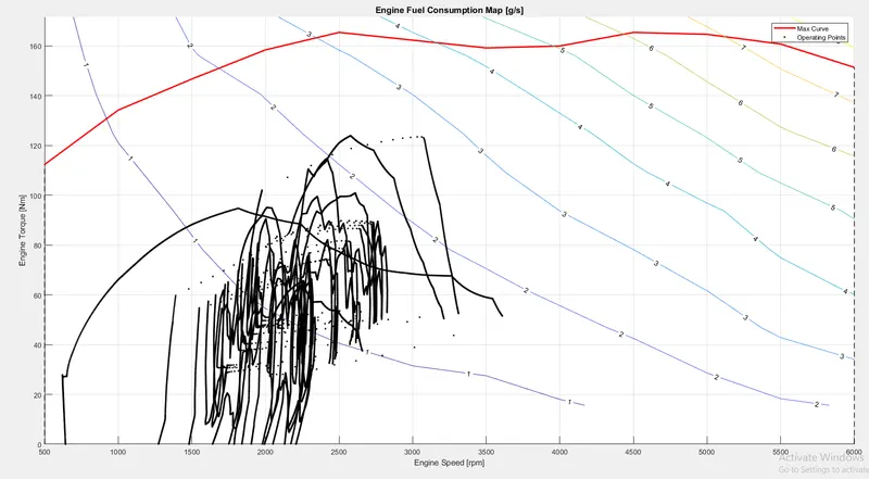
%% Plotting engine operating points on engine fuel map
figure('Name','Engine Operating Points');
hold on
grid on
title('Engine Operating Points','fontsize',12);
p1=plot(Eng_map_spd*30/pi,Eng_max_trq,'linewidth',2,'color','r');
p2=line([Eng_map_spd(end)*30/pi Eng_map_spd(end)*30/pi],[0 Eng_max_trq(end)]);
set(p2,'linewidth',1,'linestyle','--','color','k');
p3=line([Eng_map_spd(1)*30/pi Eng_map_spd(1)*30/pi],[0 Eng_max_trq(1)]);
set(p3,'linewidth',1,'linestyle','--','color','k');
[c,h] = contour(Eng_map_spd'*30/pi,Eng_map_trq,Eng_fuel_map');
clabel(c,h);
xlabel('Engine Speed [rpm]');
ylabel('Engine Torque [Nm]');
title('Engine Fuel Consumption Map [g/s]');
p4 = plot(Eng_Spd,Eng_Trq,'.','color','k');
legend([p1 p4],{'Max Curve','Operating Points'});
axis([Eng_map_spd(1)*30/pi Eng_map_spd(end)*30/pi 0 Eng_map_trq(end)]);
Figure-1
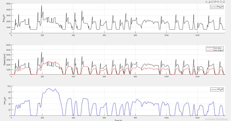
Figure-2
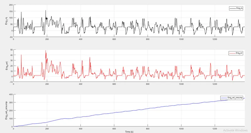
Figure-3
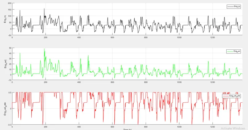
Figure-4
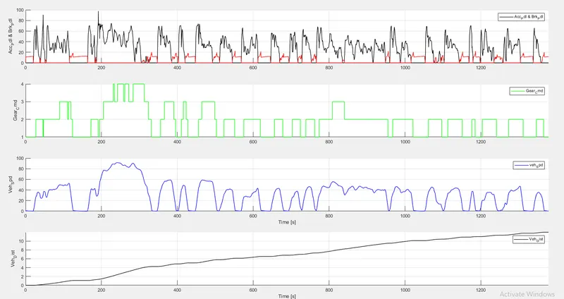
Figure-5
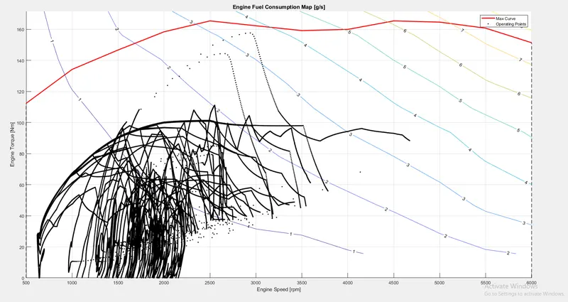
Ans) To compute the fuel economy numbers for the given vehicle (kmpl) on the urban cycle (UDDS)Also, to analyze and understand the vehicle operating points in terms of engine speed, torque, transmission speeds, and pedal positions, gear, distance traveled, etc.
Drive Cycle -2 (HWFET)
Project-1 Initial_File.m
%%%%%%%%%%%%%%%%%%%%%%%%%%%%%%%%%%%%%%%%%%%%%%%%%%%%%%%%%%%%%%%%%%%%%
%% Skill-Lync -> Hybrid Drives Development
% Project 1 - Conventional Vehicle Model
% By - Ullekh Gambhira

% Description:

%% Initialization File
% Initialization file for loading the variables for the Conventional vehicle simulation model

%% Vehicle Parameters
M = 1500;       % Vehicle weight [kg]
Cr = 0.015;     % Rolling resistance coefficient
Rw = 0.35;      % Rolling radius [m]
Cd = 0.33;      % Drag coefficient
Af = 2;         % Frontal area [m2]
rhoa = 1.225;   % Air density [kg/m3]
Vwind = 0;      % Wind velocity [kmph]
g = 9.81;       % Gravitational acceleration [m/s2]
theta = 0;      % Slope [deg]
myu_road_tire = 1; % Coefficient of friction between tire - road interface

%% Powertrain Parameters
FDR = 3.73;                         % Final Drive Ratio / Diff Ratio
DiffEff = 0.99;                     % Differential efficiency (assumed independent of operating conditions)

NumGear = 4;                        % Number of gears in transmission
TransGear = [1:NumGear];            % Transmission Gears
TransRatio = [3.06, 1.62, 1, 0.7];  % Corresponding Transmission ratios
TransEff = 0.90;                    % Transmission efficiency (assumed independent of operating conditions)

TC_SR = [0, .5, .6, .7, .8, .87, .92, .94, .96, .97, 1];   % Torque Converter Speed Ratio (Matlab default) -> TurbSpd/PumpSpd
TC_TR = [2.232, 1.5462, 1.4058, 1.2746, 1.1528, 1.0732, 1.0192, 1, 1, 1, 1];   % Torque Converter Torque Ratio (Matlab default) -> TurbTrq/PumpTrq
TC_Cf = 1e-4 * [.72558, .66322, .63463, .59042, .51331, .4144, .29287, .22444, .12186, .04386, 0]; % Torque Converter Capacity Factor (Matlab default) -> PumpTrq/PumpSpd^2 [Nm/rpm^2]

load Vehicle_Data/Engine_data_1_9L_Saturn_95kW
load Vehicle_Data/Trans_Shift_map

%% Driver Parameters
Kp = 10;                    % P gain for driver PI model
Ki = 1;                     % I gain for driver PI model
Drive_Cycle_Select = 2;     % Drive cycle selection

% Drive cycle values in m/s

if Drive_Cycle_Select == 1
    load DriveCycles/UDDS;

elseif Drive_Cycle_Select == 2
    load DriveCycles/HWFET;

elseif Drive_Cycle_Select == 3
    load DriveCycles/FTP;

elseif Drive_Cycle_Select == 4
    load DriveCycles/US06;

elseif Drive_Cycle_Select == 5
    load DriveCycles/NEDC;

elseif Drive_Cycle_Select == 6
    load DriveCycles/WLTP;

end

time_end = cyc_time(end);
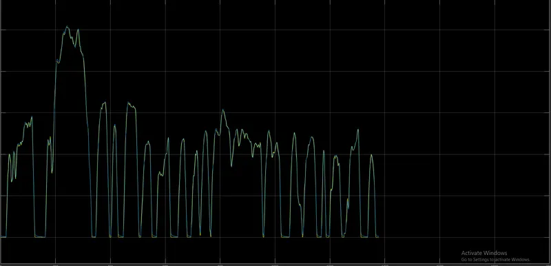
vel_end = cyc_vel(end);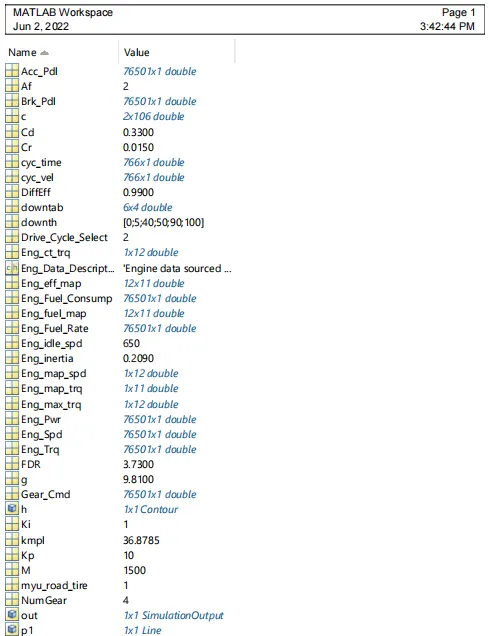
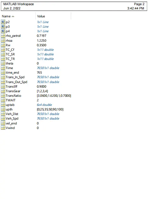
a) Vehicle Dynamics
B) Engine
Project-1 Processing_File.m
%%%%%%%%%%%%%%%%%%%%%%%%%%%%%%%%%%%%%%%%%%%%%%%%%%%%%%%%%%%%%%%%%%%%%
%% Skill-Lync -> Hybrid Drives Development
% Project 1 - Conventional Vehicle Model
% By - Ullekh Gambhira

% Description:
% The following file is to used with the Initialization file and Simulink
% results for post-processing of the data.
% The file is incomplete, has some examples of how the data is imported
% into a readable format, data analysis and plotting examples.
% Based on the project task, use commands in a similar format as given
% below, to analyse the data and generate required plots.
% You can change variable names if desired

%% Post-Processing File
%  File for post-processing the Conventional vehicle simulation model data

%% Renaming variables
Time = out.tout;
Acc_Pdl = out.Acc_Pdl;          % Accelerator pedal [%]
Brk_Pdl = out.Brk_Pdl;          % Brake pedal [%]
Gear_Cmd = out.Gear_Cmd;        % Transmission gear
Trans_In_Spd = out.Trans_In_Spd*30/pi;  % Transmission input speed [rpm]
Trans_Out_Spd = out.Trans_Out_Spd*30/pi;% Transmission output speed [rpm]
Eng_Trq = out.Eng_Trq;          % Engine brake torque [Nm]
Eng_Spd = out.Eng_Spd.*30/pi;    % Engine speed [rpm]
Eng_Fuel_Consump = out.Eng_Fuel_Consumption;    % Engine fuel consumption [g]
Veh_Dist = out.Veh_Dist/1000;   % Distance traveled by vehicle [km]
Veh_Spd = out.Veh_Spd*18/5;     % Vehicle speed [kmph]
Eng_Fuel_Rate = out.Eng_Fuel_Rate;%Engine Fuel rate

%% Data Analysis
Eng_Pwr = Eng_Spd*pi/30.*Eng_Trq/1000;   % Engine brake power [kW]
rho_petrol = 0.7197;                    % Density of petrol [kg/L]
kmpl = Veh_Dist(end)/(Eng_Fuel_Consump(end)/1000/rho_petrol);    % Fuel economy [kmpl]


%% Plotting vehicle characteristics time trace
figure(1)
subplot(3,1,1)
hold on
grid on
plot(Time,Eng_Spd, 'linewidth', 1, 'Color', 'black');
ylabel('Eng_Spd')
xlim([0, Time(end)]);
legend('Eng_Spd');
subplot(3,1,2)
hold on
grid on
plot(Time, Trans_In_Spd, 'linewidth', 1, 'Color', 'black');
plot(Time, Trans_Out_Spd, 'linewidth', 1, 'Color', 'red');
ylabel('Speed [rpm]')
xlim([0, Time(end)]);
ylim([0, 6000]);
legend('Trans Input','Trans Output');
subplot(3,1,3)
hold on
grid on
plot(Time,Veh_Spd, 'linewidth', 1, 'Color', 'blue');
xlim([0, Time(end)]);
xlabel('Time [s]');
ylabel('Veh_Spd');
legend('veh_Spd');

figure(2)
subplot(3,1,1)
hold on
grid on
plot(Time,Eng_Trq, 'linewidth', 1, 'Color', 'black');
ylabel('Eng_Trq')
xlim([0, Time(end)]);
legend('Eng_Trq');
subplot(3,1,2)
hold on
grid on
plot(Time, Eng_Pwr , 'linewidth', 1, 'Color', 'red');
ylabel('Eng_Pwr]')
xlim([0, Time(end)]);
legend('Eng_Pwr');
subplot(3,1,3)
hold on
grid on
plot(Time,Eng_Fuel_Consump, 'linewidth', 1, 'Color', 'blue');
xlim([0, Time(end)]);
xlabel('Time [s]');
ylabel('Eng_Fuel_Consump');
legend('Eng_Fuel_Consump');

figure(3)
subplot(3,1,1)
hold on
grid on
plot(Time,Eng_Trq, 'linewidth', 1, 'Color', 'black');

ylabel('Eng_Trq')
xlim([0, Time(end)]);
legend('Eng_Trq');
subplot(3,1,2)
hold on
grid on
plot(Time, Eng_Pwr , 'linewidth', 1, 'Color', 'green');
ylabel('Eng_Pwr]')
xlim([0, Time(end)]);
legend('Eng_Pwr');
subplot(3,1,3)
hold on
grid on
plot(Time,Eng_Fuel_Rate , 'linewidth', 1, 'Color', 'red');
xlim([0, Time(end)]);
xlabel('Time [s]');
ylabel('Eng_Fuel_Rate ');
legend('Eng_Fuel_Rate ');

figure(4)
subplot(4,1,1)
hold on
grid on
plot(Time,Acc_Pdl, 'linewidth', 1, 'Color', 'black');
plot(Time, Brk_Pdl, 'linewidth', 1, 'Color', 'red');
ylabel('Acc_Pdl & Brk_Pdl')
xlim([0, Time(end)]);
legend('Acc_Pdl & Brk_Pdl');
subplot(4,1,2)
hold on
grid on
plot(Time, Gear_Cmd, 'linewidth', 1, 'Color', 'green');
ylabel('Gear_Cmd')
xlim([0, Time(end)]);
legend('Gear_Cmd');
subplot(4,1,3)
hold on
grid on
plot(Time,Veh_Spd, 'linewidth', 1, 'Color', 'blue');
xlim([0, Time(end)]);
xlabel('Time [s]');
ylabel('Veh_Spd');
legend('veh_Spd');
subplot(4,1,4)
hold on
grid on
plot(Time,Veh_Dist, 'linewidth', 1, 'Color', 'black');
xlim([0, Time(end)]);
xlabel('Time [s]');
ylabel('Veh_Dist');
legend('Veh_Dist');

%% Plotting engine operating points on engine fuel map
figure('Name','Engine Operating Points');
hold on
grid on
title('Engine Operating Points','fontsize',12);
p1=plot(Eng_map_spd*30/pi,Eng_max_trq,'linewidth',2,'color','r');
p2=line([Eng_map_spd(end)*30/pi Eng_map_spd(end)*30/pi],[0 Eng_max_trq(end)]);
set(p2,'linewidth',1,'linestyle','--','color','k');
p3=line([Eng_map_spd(1)*30/pi Eng_map_spd(1)*30/pi],[0 Eng_max_trq(1)]);
set(p3,'linewidth',1,'linestyle','--','color','k');
[c,h] = contour(Eng_map_spd'*30/pi,Eng_map_trq,Eng_fuel_map');
clabel(c,h);
xlabel('Engine Speed [rpm]');
ylabel('Engine Torque [Nm]');
title('Engine Fuel Consumption Map [g/s]');
p4 = plot(Eng_Spd,Eng_Trq,'.','color','k');
legend([p1 p4],{'Max Curve','Operating Points'});
axis([Eng_map_spd(1)*30/pi Eng_map_spd(end)*30/pi 0 Eng_map_trq(end)]);
Figure-1
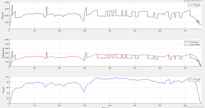
Figure-2
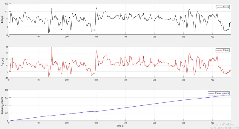
Figure-3
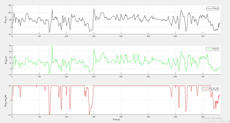
Figure-4
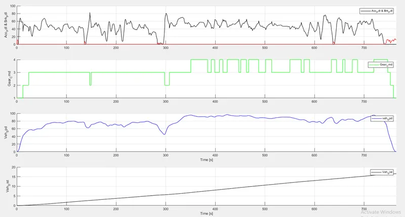
Figure-5
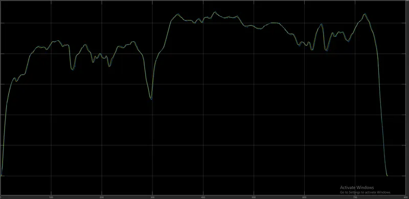
| Sl no | parameters | UDDS | HWFET |
| 1 | Time | 1369 | 765 |
| 2 | Distance | 7.663 | 16.50 |
| 3 | Speed | 44.70 | 0.350 |
| 4 | Average | 24.970 | 36.875 |