AIM:
The main goal of this project is to get familiar with the modeling process, writing scripts in Matlab, modeling in Simulink, analyzing data and generating plots.
Task:
The task of this project is to compute the fuel economy numbers for the given vehicle (kmpl) on the urban cycle (UDDS) and highway cycle (HWFET). Also, to analyze and understand the vehicle operating
points in terms of engine speed, torque, transmission speeds, pedal positions, gear, distance traveled, etc
PROCEDURE:
1) Load the Project1 folder as the Current Folder in Matlab.
2) Run the “Project1_InitFile.m” Matlab script.
3) The provided vehicle Simulink model “Project1_VehicleModel.slx” is incomplete. The engine and vehicle dynamics block contents have been deleted. Build the Simulink blocks by referring to the course lecture and example block images provided. You can run the model and analyze the results using a ‘Scope’ for debugging.
4) Add additional ‘To Workspace’ blocks for transferring the desired Simulink vehicle data into the Matlab workspace.
5) Modify the “Project1_ProcessingFile.m” as per the desired plots and required calculations.
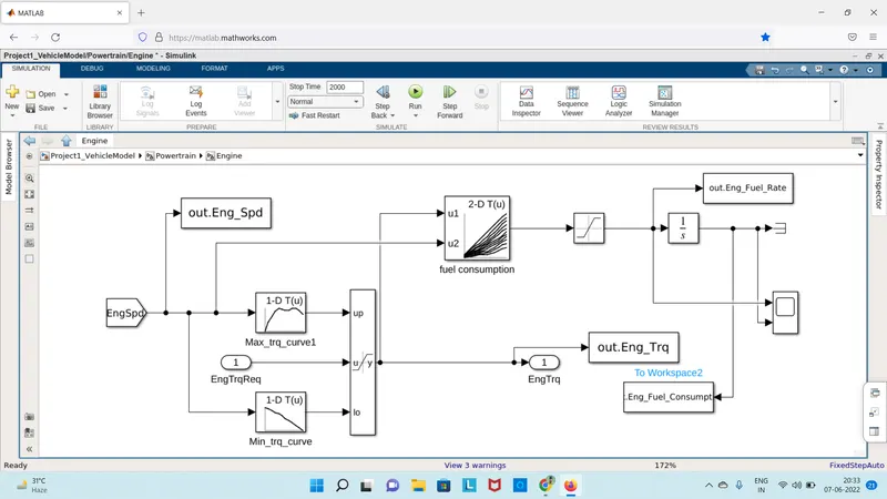
ENGINE BLOCK:
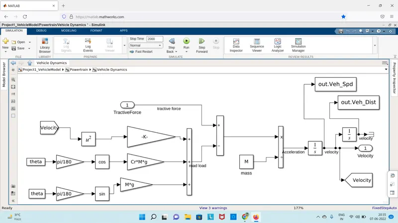
VEHICLE DYNAMICS:
Now running the “Project1_InitFile.m” Matlab script.
%% Skill-Lync -> Hybrid Drives Development
% Project 1 - Conventional Vehicle Model
% By - Ullekh Gambhira
% Description:
%% Initialization File
% Initialization file for loading the variables for the Conventional vehicle simulation model
%% Vehicle Parameters
M = 1500; % Vehicle weight [kg]
Cr = 0.015; % Rolling resistance coefficient
Rw = 0.35; % Rolling radius [m]
Cd = 0.33; % Drag coefficient
Af = 2; % Frontal area [m2]
rhoa = 1.225; % Air density [kg/m3]
Vwind = 0; % Wind velocity [kmph]
g = 9.81; % Gravitational acceleration [m/s2]
theta = 0; % Slope [deg]
myu_road_tire = 1; % Coefficient of friction between tire - road interface
%% Powertrain Parameters
FDR = 3.73; % Final Drive Ratio / Diff Ratio
DiffEff = 0.99; % Differential efficiency (assumed independent of operating conditions)
NumGear = 4; % Number of gears in transmission
TransGear = [1:NumGear]; % Transmission Gears
TransRatio = [3.06, 1.62, 1, 0.7]; % Corresponding Transmission ratios
TransEff = 0.90; % Transmission efficiency (assumed independent of operating conditions)
TC_SR = [0, .5, .6, .7, .8, .87, .92, .94, .96, .97, 1]; % Torque Converter Speed Ratio (Matlab default) -> TurbSpd/PumpSpd
TC_TR = [2.232, 1.5462, 1.4058, 1.2746, 1.1528, 1.0732, 1.0192, 1, 1, 1, 1]; % Torque Converter Torque Ratio (Matlab default) -> TurbTrq/PumpTrq
TC_Cf = 1e-4 * [.72558, .66322, .63463, .59042, .51331, .4144, .29287, .22444, .12186, .04386, 0]; % Torque Converter Capacity Factor (Matlab default) -> PumpTrq/PumpSpd^2 [Nm/rpm^2]
load Vehicle_Data/Engine_data_1_9L_Saturn_95kW
load Vehicle_Data/Trans_Shift_map
%% Driver Parameters
Kp = 10; % P gain for driver PI model
Ki = 1; % I gain for driver PI model
Drive_Cycle_Select = 1; % Drive cycle selection
% Drive cycle values in m/s
if Drive_Cycle_Select == 1
load DriveCycles/UDDS.MAT;
elseif Drive_Cycle_Select == 2
load DriveCycles/HWFET;
elseif Drive_Cycle_Select == 3
load DriveCycles/FTP;
elseif Drive_Cycle_Select == 4
load DriveCycles/US06;
elseif Drive_Cycle_Select == 5
load DriveCycles/NEDC;
elseif Drive_Cycle_Select == 6
load DriveCycles/WLTP;
end
time_end = cyc_time(end);
vel_end = cyc_vel(end);
After running this Project1_InitFile.m script we need to run simulink model (Project1_VehicleModel.slx) then we need to run Project1_ProcessingFile.m
%% Skill-Lync -> Hybrid Drives Development
% Project 1 - Conventional Vehicle Model
% By - Ullekh Gambhira
% Description:
%% Renaming variables
Time = out.tout;
Acc_Pdl = out.Acc_Pdl; % Accelerator pedal [%]
Brk_Pdl = out.Brk_Pdl; % Brake pedal [%]
Gear_Cmd = out.Gear_Cmd; % Transmission gear
Trans_In_Spd = out.Trans_In_Spd*30/pi; % Transmission input speed [rpm]
Trans_Out_Spd = out.Trans_Out_Spd*30/pi;% Transmission output speed [rpm]
Eng_Trq = out.Eng_Trq; % Engine brake torque [Nm]
Eng_Spd = out.Eng_Spd*30/pi; % Engine speed [rpm]
Eng_Fuel_Consump = out.Eng_Fuel_Consumption; % Engine fuel consumption [g]
Veh_Dist = out.Veh_Dist/1000; % Distance traveled by vehicle [km]
Veh_Spd = out.Veh_Spd*18/5; % Vehicle speed [kmph]
Eng_Fuel_Rate = out.Eng_Fuel_Rate; % engine fuel rate gm/sec
%% Data Analysis
Eng_Pwr = Eng_Spd.*pi/30.*Eng_Trq/1000; % Engine brake power [kW]
rho_petrol = 0.7197; % Density of petrol [kg/L]
kmpl = Veh_Dist(end)/(Eng_Fuel_Consump(end)/1000/rho_petrol); % Fuel economy [kmpl]
%% Plotting vehicle characteristics time trace
figure()
subplot(5,1,1)
hold on
grid on
plot(Time, Acc_Pdl, 'linewidth', 1, 'Color', 'black');
plot(Time, Brk_Pdl, 'linewidth', 1, 'Color', 'red');
ylabel('Pedal [%]')
xlim([0, Time(end)]);
legend('Accel','Brake');
subplot(5,1,2)
hold on
grid on
plot(Time, Trans_In_Spd, 'linewidth', 1, 'Color', 'black');
plot(Time, Trans_Out_Spd, 'linewidth', 1, 'Color', 'red');
ylabel('Speed [rpm]')
xlim([0, Time(end)]);
ylim([0, 6000]);
legend('Trans Input','Trans Output');
subplot(5,1,3)
hold on
grid on
plot(Time, Gear_Cmd, 'linewidth', 1, 'Color', 'black');
xlim([0, Time(end)]);
xlabel('Time [s]');
ylabel('Gear');
subplot(5,1,4)
hold on
grid on
plot(Time,Act_Spd,'LineWidth',1,'Color','black');
plot(Time,Veh_Spd,'LineWidth',1,'Color','red');
xlim([0,Time(end)]);
xlabel('Time[sec]');
ylabel('Speed(kmph)');
legend('Actual speed','Vehicle speed')
subplot(5,1,5)
hold on
grid on
plot(Time,Veh_Dist,'LineWidth',1,'Color','black');
xlim([0,Time(end)]);
xlabel('Time[sec]');
ylabel('Distance(km)');
legend('distance')
figure(2)
subplot(4,1,1)
plot(Time,Eng_Trq,'linewidth',1,'color','black')
xlim([0,Time(end)]);
xlabel('Time[sec]');
ylabel('Torque[Nm]');
hold on
grid on
subplot(4,1,2)
plot(Time,Eng_Pwr,'linewidth',1,'color','black')
xlim([0,Time(end)]);
xlabel('Time[sec]');
ylabel('Power[KW]');
hold on
grid on
subplot(4,1,3)
plot(Time,Eng_Fuel_Rate,'linewidth',1,'color','black')
xlim([0,Time(end)]);
xlabel('Time[sec]');
ylabel('Fuel rate[gm/sec');
hold on
grid on
subplot(4,1,4)
plot(Time,Eng_Fuel_Consump,'linewidth',1,'color','black')
xlim([0,Time(end)]);
xlabel('Time[sec]');
ylabel('Fuel consumption[gm]');
hold on
grid on
%% Plotting engine operating points on engine fuel map
figure( 'Name','Engine Operating Points');
hold on
grid on
title('Engine Operating Points','fontsize',12);
p1=plot(Eng_map_spd*30/pi,Eng_max_trq,'linewidth',2,'color','r');
p2=line([Eng_map_spd(end)*30/pi Eng_map_spd(end)*30/pi],[0 Eng_max_trq(end)]);
set(p2,'linewidth',1,'linestyle','--','color','k');
p3=line([Eng_map_spd(1)*30/pi Eng_map_spd(1)*30/pi],[0 Eng_max_trq(1)]);
set(p3,'linewidth',1,'linestyle','--','color','k');
[c,h] = contour(Eng_map_spd'*30/pi,Eng_map_trq,Eng_fuel_map');
clabel(c,h);
xlabel('Engine Speed [rpm]');
ylabel('Engine Torque [Nm]');
title('Engine Fuel Consumption Map [g/s]');
p4 = plot(Eng_Spd,Eng_Trq,'.','color','k');
legend([p1 p4],{'Max Curve','Operating Points'});
axis([Eng_map_spd(1)*30/pi Eng_map_spd(end)*30/pi 0 Eng_map_trq(end)]);
PLOTS FOR UDDS:
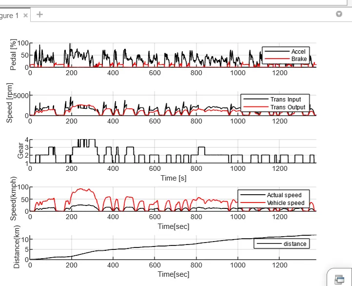
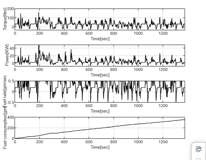
- From the 5.1.1 plot we can observe that acelerator and brake are evenly used to drive the vehicle. In this case both are non linear.
- From the 5.1.2 plot transmission input and output also non linear and normally transmission input is more compare to transmission output speed due to engine operating speed. The time trace to reach that speed is high for input and output.
- From 5.1.3 plot gear shifting is frequently changes due to uneven speeds of drive cycle,same thing we can see in the plot.
- From the plot 5.1.4 actual speed and vehicle speeds are varying in different speeds. The difference between these two is very high.
- From the plot 5.1.5 normally distance increase with time increase.
- From the 4.1.1 , 4.1.2 and 4.1.3 we can see that engine torque, engine power and engine fuel rate are non linear with time they are varying with the time.
- From the 4.1.4 plot we can see fuel consumption increasing with time.
ENGINE OPERATING AND FUEL EFFICIENCY MAP OF UDDS:
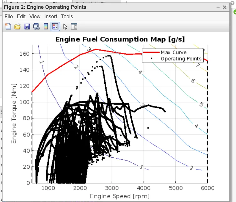
- Engine fuel efficiency map is generated using Engine torque and Engine speed.
- As Engine speed increases engine torque is also inceasing.
PLOTS FOR HWFET:
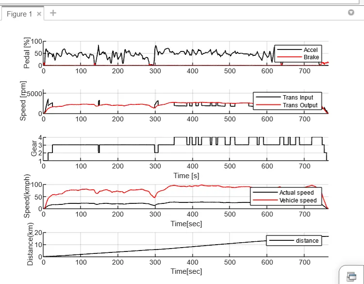
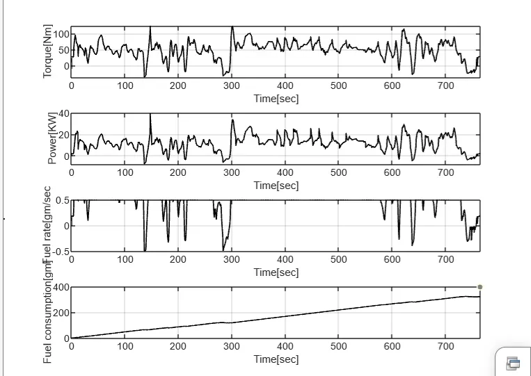
- From the 5.1.1 plot we can observe that acelerator and brake are evenly used to drive the vehicle. In this case both are non linear.
- From the 5.1.2 plot transmission input and output also non linear and normally transmission input is more compare to transmission output speed due to engine operating speed. The time trace to reach that speed is high for input and output.
- From 5.1.3 plot gear shifting is frequently changes due to uneven speeds of drive cycle,same thing we can see in the plot.
- From the plot 5.1.4 actual speed and vehicle speeds are varying in different speeds. The difference between these two is very high.
- From the plot 5.1.5 normally distance increase with time increase.
- From the 4.1.1 , 4.1.2 and 4.1.3 we can see that engine torque, engine power and engine fuel rate are non linear with time they are varying with the time.
- From the 4.1.4 plot we can see fuel consumption increasing with time.
ENGINE OPERATING AND FUEL EFFICIENCY MAP OF HWFET:
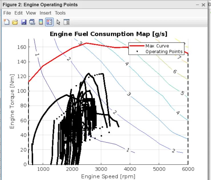
- Engine fuel efficiency map is generated using Engine torque and Engine speed.
- As Engine speed increases engine torque is also inceasing.