AIM:
By using the data provided with varibles in "Project1_initFile.m" for vehicle model to complete the deleted model contents of simulink model "Project1_vehiclemodel.slx" and to load data to workspace and execute the file "Project1_processingfile.m" with the data loaded back to workspace from the model and complete the below task for UDDS and HWFET drive cycles
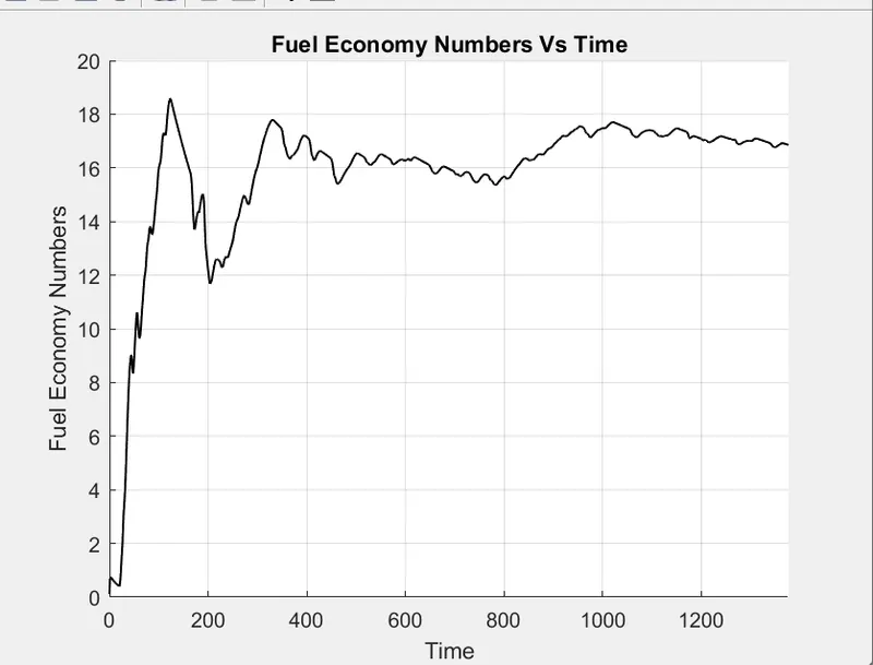
1. Tabulate fuel economy numbers (kmpl) for UDDS & HWFET.
2. Plot Time trace for Engine, Transmission Input, Transmission Output Wheel speed in One plot.
3. Plot Engine Torque, Engine Power, Fuel rate and Fuel consumption using sub-plots.
4. Plot Acceleration & Brake pedals, Gear command, Vehicle desired and actual speed, Vehicle distance.
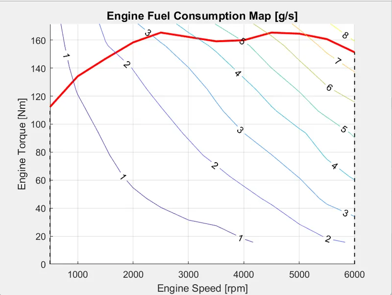
5. Plot Enginge operating points on Engine fuel map.
DESCRIPTION:
1.CODE FOR VARIABLES OF MODEL FROM FILE:
%% Skill-Lync -> Hybrid Drives Development
% Project 1 - Conventional Vehicle Model
% By - Ullekh Gambhira
% Description:
%% Initialization File
% Initialization file for loading the variables for the Conventional vehicle simulation model
%% Vehicle Parameters
M = 1500; % Vehicle weight [kg]
Cr = 0.015; % Rolling resistance coefficient
Rw = 0.35; % Rolling radius [m]
Cd = 0.33; % Drag coefficient
Af = 2; % Frontal area [m2]
rhoa = 1.225; % Air density [kg/m3]
Vwind = 0; % Wind velocity [kmph]
g = 9.81; % Gravitational acceleration [m/s2]
theta = 0; % Slope [deg]
myu_road_tire = 1; % Coefficient of friction between tire - road interface
%% Powertrain Parameters
FDR = 3.73; % Final Drive Ratio / Diff Ratio
DiffEff = 0.99; % Differential efficiency (assumed independent of operating conditions)
NumGear = 4; % Number of gears in transmission
TransGear = [1:NumGear]; % Transmission Gears
TransRatio = [3.06, 1.62, 1, 0.7]; % Corresponding Transmission ratios
TransEff = 0.90; % Transmission efficiency (assumed independent of operating conditions)
TC_SR = [0, .5, .6, .7, .8, .87, .92, .94, .96, .97, 1]; % Torque Converter Speed Ratio (Matlab default) -> TurbSpd/PumpSpd
TC_TR = [2.232, 1.5462, 1.4058, 1.2746, 1.1528, 1.0732, 1.0192, 1, 1, 1, 1]; % Torque Converter Torque Ratio (Matlab default) -> TurbTrq/PumpTrq
TC_Cf = 1e-4 * [.72558, .66322, .63463, .59042, .51331, .4144, .29287, .22444, .12186, .04386, 0]; % Torque Converter Capacity Factor (Matlab default) -> PumpTrq/PumpSpd^2 [Nm/rpm^2]
load Vehicle_Data/Engine_data_1_9L_Saturn_95kW
load Vehicle_Data/Trans_Shift_map
%% Driver Parameters
Kp = 10; % P gain for driver PI model
Ki = 1; % I gain for driver PI model
Drive_Cycle_Select = 1; % Drive cycle selection
% Drive cycle values in m/s
if Drive_Cycle_Select == 1
load DriveCycles/UDDS;
elseif Drive_Cycle_Select == 2
load DriveCycles/HWFET;
elseif Drive_Cycle_Select == 3
load DriveCycles/FTP;
elseif Drive_Cycle_Select == 4
load DriveCycles/US06;
elseif Drive_Cycle_Select == 5
load DriveCycles/NEDC;
elseif Drive_Cycle_Select == 6
load DriveCycles/WLTP;
end
time_end = cyc_time(end);
vel_end = cyc_vel(end);
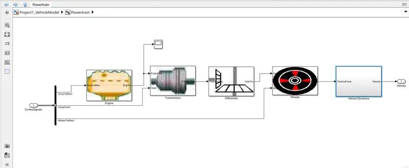
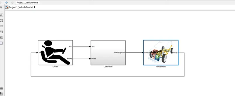
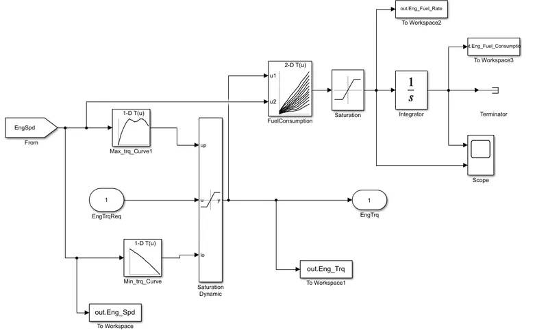
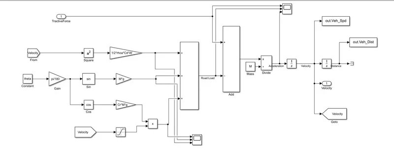
2.DELETED MODEL COMPLETED:
ENGINE COMPONENT IN POWERTRAIN OF VEHICLE MODEL:
VEHICLE DYNAMICS COMPONENT IN POWER TRAIN:
3.CODE FOR DESIRED PLOTS FROM THE SIMULINK MODEL:
CODE FOR RENAMING VARIABLES:
%% Renaming variables
Time = out.tout;
Acc_Pdl = out.Acc_Pdl; % Accelerator pedal [%]
Brk_Pdl = out.Brk_Pdl; % Brake pedal [%]
Gear_Cmd = out.Gear_Cmd; % Transmission gear
Trans_In_Spd = out.Trans_In_Spd*30/pi; % Transmission input speed [rpm]
Trans_Out_Spd = out.Trans_Out_Spd*30/pi;% Transmission output speed [rpm]
Eng_Trq = out.Eng_Trq; % Engine brake torque [Nm]
Eng_Spd = out.Eng_Spd*30/pi; % Engine speed [rpm]
Eng_Fuel_Consump = out.Eng_Fuel_Consumption; % Engine fuel consumption [g]
Veh_Dist = out.Veh_Dist/1000; % Distance traveled by vehicle [km]
Veh_Spd = out.Veh_Spd*18/5; % Vehicle speed [kmph]
%% Data Analysis
Eng_Pwr = Eng_Spd*pi/30*Eng_Trq/1000; % Engine brake power [kW]
rho_petrol = 0.7197; % Density of petrol [kg/L]
kmpl = Veh_Dist(end)/(Eng_Fuel_Consump(end)/1000/rho_petrol); % Fuel economy [kmpl]
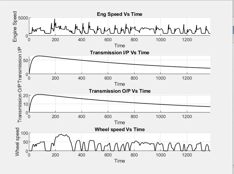
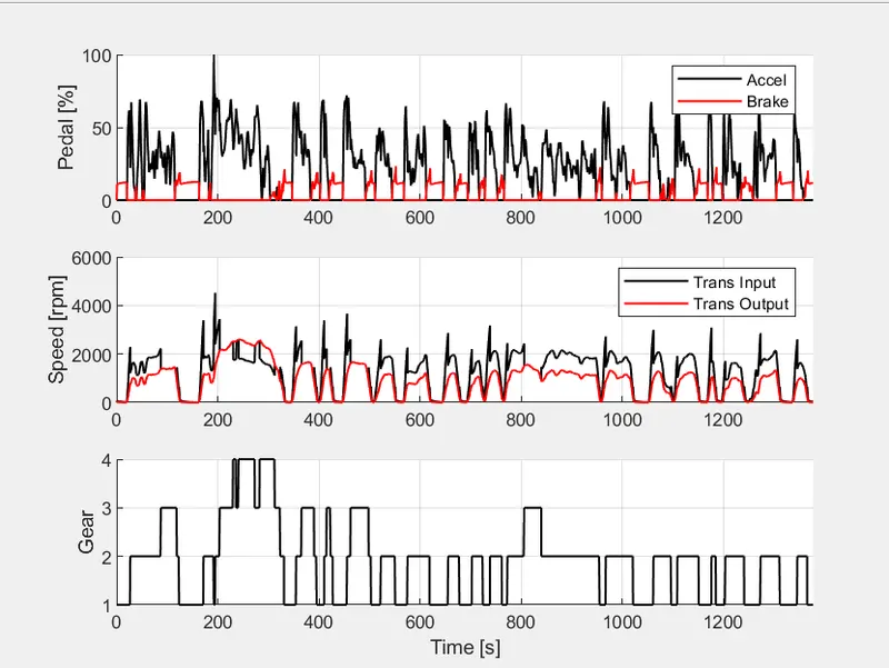
CODE TO PLOT TIME TRACE FOR ENGINE, TRANSMISSION I/P, TRANSMISSION O/P, WHEEL SPEED IN ONE PLOT:
%% Plotting vehicle characteristics time trace
figure()
subplot(3,1,1)
hold on
grid on
plot(Time, Acc_Pdl, 'linewidth', 1, 'Color', 'black');
plot(Time, Brk_Pdl, 'linewidth', 1, 'Color', 'red');
ylabel('Pedal [%]')
xlim([0, Time(end)]);
legend('Accel','Brake');
subplot(3,1,2)
hold on
grid on
plot(Time, Trans_In_Spd, 'linewidth', 1, 'Color', 'black');
plot(Time, Trans_Out_Spd, 'linewidth', 1, 'Color', 'red');
ylabel('Speed [rpm]')
xlim([0, Time(end)]);
ylim([0, 6000]);
legend('Trans Input','Trans Output');
subplot(3,1,3)
hold on
grid on
plot(Time, Gear_Cmd, 'linewidth', 1, 'Color', 'black');
xlim([0, Time(end)]);
xlabel('Time [s]');
ylabel('Gear');
CODE FOR PLOTTING ENGINE OPERATING POINTS ON ENGINE FUEL MAP:
%% Plotting engine operating points on engine fuel map
figure('Name','Engine Operating Points');
hold on
grid on
title('Engine Operating Points','fontsize',12);
p1=plot(Eng_map_spd*30/pi,Eng_max_trq,'linewidth',2,'color','r');
p2=line([Eng_map_spd(end)*30/pi Eng_map_spd(end)*30/pi],[0 Eng_max_trq(end)]);
set(p2,'linewidth',1,'linestyle','--','color','k');
p3=line([Eng_map_spd(1)*30/pi Eng_map_spd(1)*30/pi],[0 Eng_max_trq(1)]);
set(p3,'linewidth',1,'linestyle','--','color','k');
[c,h] = contour(Eng_map_spd'*30/pi,Eng_map_trq,Eng_fuel_map');
clabel(c,h);
xlabel('Engine Speed [rpm]');
ylabel('Engine Torque [Nm]');
title('Engine Fuel Consumption Map [g/s]');
p4 = plot(Eng_Spd,Eng_Trq,'.','color','k');
legend([p1 p4],{'Max Curve','Operating Points'});
axis([Eng_map_spd(1)*30/pi Eng_map_spd(end)*30/pi 0 Eng_map_trq(end)]);
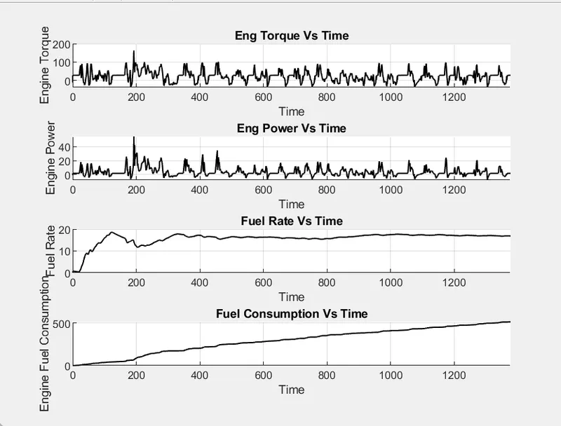
CODE TO PLOT ENGINE TORQUE, ENGINE POWER, FUEL RATE & FUEL CONSUMPTION USING SUB-PLOTS:
figure()
subplot(4,1,1)
hold on
grid on
plot(Eng_Trq, 'linewidth', 1, 'Color', 'black');
xlim([0, Time(end)]);
xlabel('Time');
ylabel('Engine Torque');
title('Eng Torque Vs Time');
subplot(4,1,2)
hold on
grid on
plot(Eng_Pwr, 'linewidth', 1, 'Color', 'black');
xlim([0, Time(end)]);
xlabel('Time');
ylabel('Engine Power');
title('Eng Power Vs Time');
subplot(4,1,3)
hold on
grid on
plot(kmpl, 'linewidth', 1, 'Color', 'black');
xlim([0, Time(end)]);
xlabel('Time');
ylabel('Fuel Rate');
title('Fuel Rate Vs Time');
subplot(4,1,4)
hold on
grid on
plot(Eng_Fuel_Consump, 'linewidth', 1, 'Color', 'black');
xlim([0, Time(end)]);
xlabel('Time');
ylabel('Engine Fuel Consumption');
title('Fuel Consumption Vs Time');
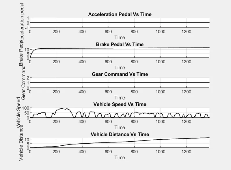
CODE FOR ACCELERATION & BRAKE PEDAL, GEAR COMMAND, VEHICLE SPEED & VEHICLE DITANCE:
figure()
subplot(5,1,1)
hold on
grid on
plot(Acc_Pdl, 'linewidth', 1, 'Color', 'black');
xlim([0, Time(end)]);
xlabel('Time');
ylabel('Acceleration pedal');
title('Acceleration Pedal Vs Time');
subplot(5,1,2)
hold on
grid on
plot(Brk_Pdl, 'linewidth', 1, 'Color', 'black');
xlim([0, Time(end)]);
xlabel('Time');
ylabel('Brake Pedal');
title('Brake Pedal Vs Time');
subplot(5,1,3)
hold on
grid on
plot(Gear_Cmd, 'linewidth', 1, 'Color', 'black');
xlim([0, Time(end)]);
xlabel('Time');
ylabel('Gear Command');
title('Gear Command Vs Time');
subplot(5,1,4)
hold on
grid on
plot(Veh_Spd, 'linewidth', 1, 'Color', 'black');
xlim([0, Time(end)]);
xlabel('Time');
ylabel('Vehicle Speed');
title('Vehicle Speed Vs Time');
subplot(5,1,5)
hold on
grid on
plot(Veh_Dist, 'linewidth', 1, 'Color', 'black');
xlim([0, Time(end)]);
xlabel('Time');
ylabel('Vehicle Distance');
title('Vehicle Distance Vs Time');
RESULTS:
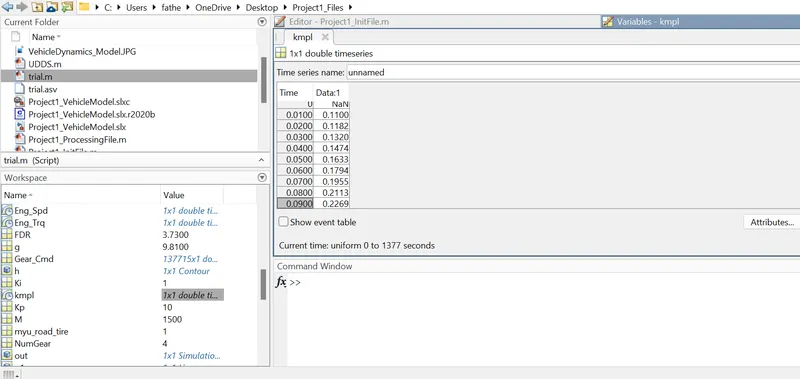
1.TABULATE FUEL ECONOMY NUMBERS(kmpl) FOR UDDS & HWFET:
Data for fuel economy numbers for UDDS and HEFET from the model executed
2.PLOT TIME TRACE FOR ENGINE, TRANSMISSION I/P, TRANSMISSION O/P, WHEEL SPEED IN ONE PLOT:
Engine speed in rpm varies from 0-5000rpm and transmission input is proportional with transmission output, Wheel speed varies from 0 to 100 with time which shows that the drive cycle is UDDS and in between the drive cycle is HWFET and keeps in varying.
3.PLOT ENGINE TORQUE, ENGINE POWER, FUEL RATE & FUEL CONSUMPTION USING SUB-PLOTS:
Here engine torque and Engine Power keeps on varying proportionally with time with increase in engine torque the power of the engine increase and decreases. Upon the usage of Engine torque and Engine POwer the fuel consumption is almost constant with increase in time and fuel consumption keeps on gradually increasing with respect to time which shows that the vehicle is in constant motion either is UDDS or HWFET drive cycle.
4.PLOT FOR ACCELERATION & BRAKE PEDAL, GEAR COMMAND, VEHICLE SPEED & VEHICLE DITANCE:
This shows that vehicle starts from speed of 0 and covers a distance, here with increase in time the distance covered by vehicle is gradually increasing which shows that vehicle is in continous motion either its a UDDS or HWFET drive cycle. Vehicle speed with time keeps on varying between 0-100mph which is the combination of both UDDS & HWFET cycle, for UDDS cycle the vehicle nomial speed is <31.5kmph and for HWFET the nominal speed is <60kmph given by the data from American institute. Gear command is 1 which indicates that vehicle is in continous motion either its UDDS or HWFET. Brake pedal and acceleration pedal is used accordingly to the drive cycle.
5.PLOTTING ENGINE OPERATING POINTS ON ENGINE FUEL MAP:
This shows that with increase in engine speed the torque of engine increases till 2000rpm which shows the vehicle starts from approximately 120Nm and upon the conditions of UDDS and HWFET they torque of the engine varies between certain limits of 110-160Nm.
CONCLUSION:
Thus, The characteristics for vehicle drive cycles of UDDS & HWFET has been studied successfully and desired plots are generated up on the given task.