Challenge

Project 1

SShivaprasad Thirandasu9 May 2022

Development of a forward energy-based fuel consumption model of a conventional vehicle.

Aim:

> The main goal of this project is to get familiar with the modeling process, writing scripts in Matlab, modeling in Simulink, analyzing data and generating plots.

>The project is to compute the fuel economy numbers for the given vehicle (kmpl) on the urban cycle (UDDS) and highway cycle (HWFET). Also, to analyze and understand the vehicle operating points in terms of engine speed, torque, transmission speeds, pedal positions, gear, distance traveled, etc.

>By using 'Project1_ProcessingFile.m' which is provided in the Matlab script used to analyze this data and to generate plots

Procedure:

1)Tabulate the fuel economy numbers (kmpl) for UDDS and HWFET cycle. This forms the baseline numbers for comparing with the future hybrid version.

2) Plot the time trace for engine, transmission input, transmission output and wheel speed on one plot.

3) Plot engine torque, engine power, fuel rate and fuel consumption using subplots.

4) Plot accelerator and brake pedal, gear command, vehicle desired and actual speed, vehicle distance using subplots.

5)Plot the engine operating points on the engine fuel map.

6)Write down appropriate brief comments on each of these plots, describing the vehicle behavior throughout the drive cycle.

7)Generate the plots for both drive cycles

Forward Energy-Based Fuel Consumption Model:

>A forward-facing vehicle model features a driver model that provides torque demand in the form of desired ICE torque and brake torque, to meet the speed trace from a drivecycle.

>A basic driver model typically uses one or more Proportional-Integral (PI) controllers to achieve the torque demand, with reference to the desired speed trace. This is discussed further in the next section. The torque produced by the ICE propagates through the transmission and final drive ratios, before ending up as torque applied at the wheels.

>This is then exerted to the vehicle mass via force on the tyre contact patch. The vehicle speed that results from the applied force is propagated back through the drivetrain, and returns to the ICE as angular velocity at the crankshaft. Brake torque is applied directly at the wheels.

Forward Vehicle Modelling

>Forward-facing models provide insight into the vehicle model drivability, and it captures the limits of the physical system. It also makes control development and implementation on HIL systems easie.

>This vehicle model used in this investigation features a conventional powertrain with an internal combustion engine, clutch, manual transmission, and final drive. Simulations that were carried out have indicated that there is minimal effect on the optimal cost with regards to variations in the driver model sensitivity.

>This opens up the possibility of using forward- facing models for the purpose of powertrain component sizing. Optimising powertrain component size for desired vehicle class and usage profile is beneficial for reducing tail pipe emissions.

Simulink Modelling:

Matlab Script:

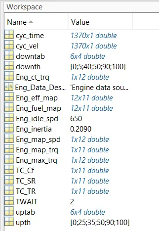
An matlab script is created to load all the data need to run and post-process the simulink model.

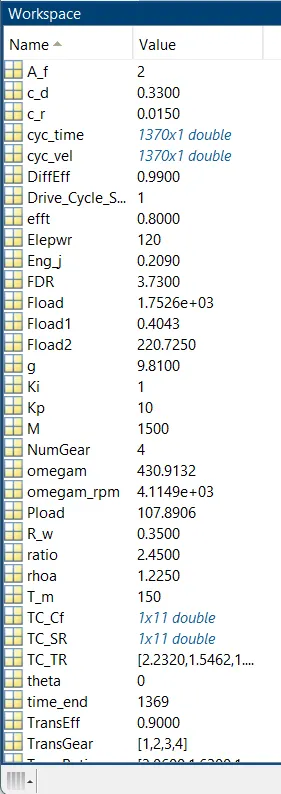
>Here all the file are loaded into the workspace for the running of simulink model.

clear all

close all

clc

%Vehicle Parameters

M = 1500; %vehicle weight(kg)

c_d= 0.33; %Drag coefficient

A_f = 2; % Forntal_Area (m^2)

rhoa =1.225; % AirDensity (kg/m^3)

c_r = 0.015; %Rolling_Resistance Coefficients

g=9.81;

theta=0;

V_h=0;

T_m=150;

efft=0.8;

ratio=2.45;

R_w=0.35; %Rolling Radius

myu_road_tire=1; % coefficient of fricition

Vveh=sqrt(efft*ratio/R_w*T_m-c_r*M*g)*2/rhoa/A_f/c_d;

Vveh_kmph=Vveh*18/5;

Fload=1/2*rhoa*c_d*A_f*(Vveh+V_h)^2+c_r*M*g*cosd(theta)+M*g*sind(theta);

omegam=ratio*Vveh/R_w;

omegam_rpm=omegam*30/pi;

% powertrain parameters

FDR=3.73; %Final Drive ratio/ Diff ratio

DiffEff=0.99; % Differential efficiency

NumGear=4; % Number of gears in transmission

TransGear=1:NumGear; % Transmission Gears

TransRatio=[3.06,1.62,1,0.7]; % corresponding Transmission ratios

TransEff=0.90; % Transmission Efficiency

TC_SR=[0,0.5,0.6,0.7,0.8,0.87,0.92,0.94,0.96,0.97,1]; % Torque Converstion speed ratio

TC_TR=[2.232,1.5462,1.4058,1.2746,1.1528,1.0732,1.0192,1,1,1];% Torque Convertion

TC_Cf = 1e-4 * [.72558, .66322, .63463, .59042, .51331, .4144, .29287, .22444, .12186, .04386, 0]; % Torque Converter

Capacity Factor (Matlab default) -> PumpTrq/PumpSpd^2 [Nm/rpm^2]

Eng_j=0.209; % Engine rotational inertia (kgm^2)

%Tm=150; % Motor Torque(Nm)

%efft=0.8; % Transmission Efficiency

Elepwr=120; % volts

%% Driver Parameters

Kp = 10; % P gain for driver PI model

Ki = 1; % I gain for driver PI model

Drive_Cycle_Select = 1; % Drive cycle selection

% Drive cycle values in m/s

if Drive_Cycle_Select == 1

load DriveCycles/UDDS;

elseif Drive_Cycle_Select == 2

load DriveCycles/HWFET;

elseif Drive_Cycle_Select == 3

load DriveCycles/FTP;

elseif Drive_Cycle_Select == 4

load DriveCycles/US06;

elseif Drive_Cycle_Select == 5

load DriveCycles/NEDC;

elseif Drive_Cycle_Select == 6

load DriveCycles/WLTP;

end

time_end = cyc_time(end);

vel_end = cyc_vel(end);

>> By running the file all the data loaded into the workspace

>> The Drive cycel is loaded into the workspace

1.UDDS

2.HWFET

3.FTP

4.US06

5.NEDC

6.WLTP

>All the given file are loaded into the workspace

SIMULINK MODEL:

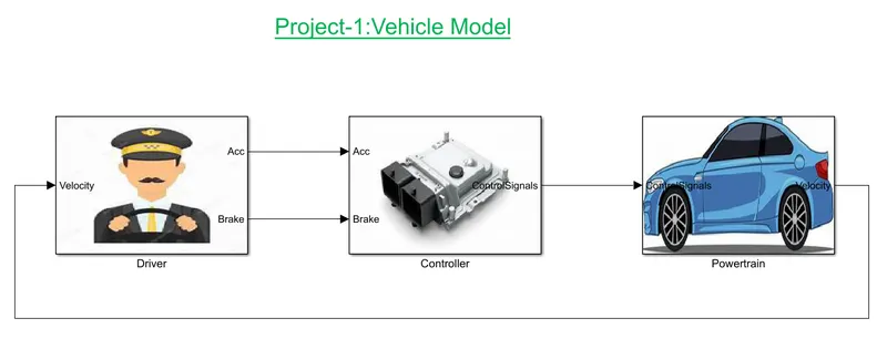
>Here the simulink main model contains 3Subsystems such as Driver,Controller,and Powertrain.

> Now we are goning in deatilly by each block how it functions and simulates the data.

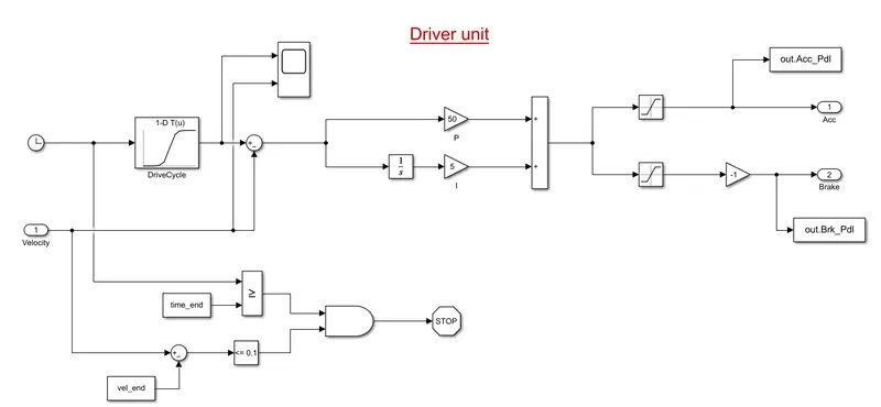
1.Driver Model:

>Driver model which takes velocity as input and the PI controller generates the Acceleration and Brake as outputs for the required vehicle speed.

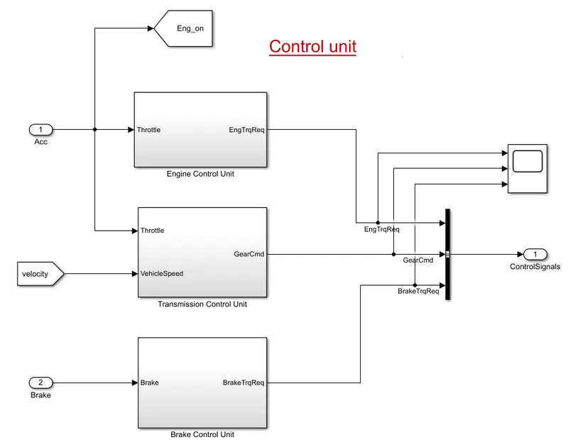
2.Contoller unit:

> The aaceleration ,velocity,Brake torque are given as inputs to the model,and all the signals are scoped in scope.

Engine control unit:

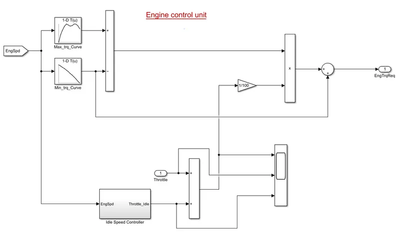
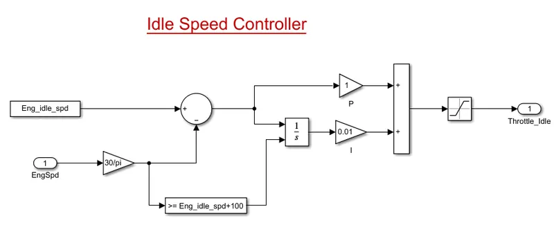
>The Engine control unit consists of another susbsystem as idle speed controller

>The Engine control unit compares engine speed with the maximum torque and minimum torque curves of the look up tables and gives requires torque to the engine block.

>The throttlr input is combined with idle speed throttr and gains with the torqueboutput from the look up table to estimate the torque input required for the engine.

Transmissoin Control Unit:

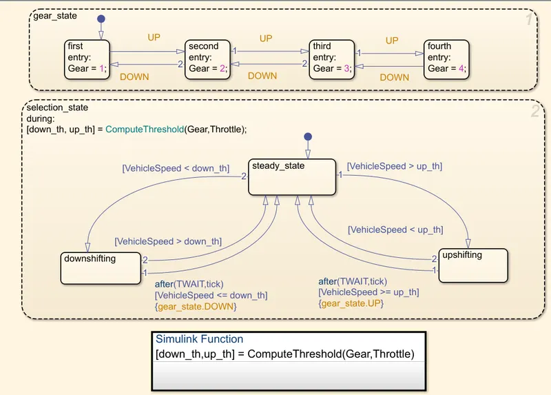
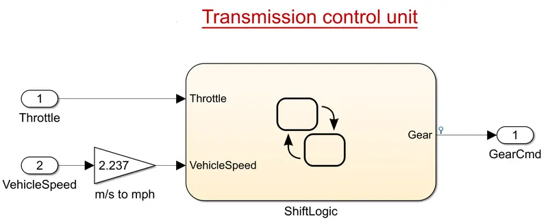
> This block controls the the gearr shifiting using the study flow variable chart.

> The gear shifiting is controlled according to the vehicle speed and throttle input.

>The gera coomand passes the signal to the transmissoin block to select the desired gear ratio.

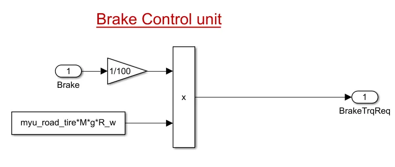
Brake Control Unit:

>This unit produces the brake torque according to the brake pedal input given and passes the brake torque in to the wheels.

Powertraim Model:

>Here it includes the Engine,Transmission.Differential,Wheels and Vehicle dynamics subsystems.

> It converts the power of engine to the vehicle's movement.

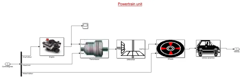
>here all these subsytems are connected to the Signal Bus connector which gives the required signals when required to the model.Input as control signal and output as velocity.

Engine:

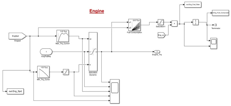
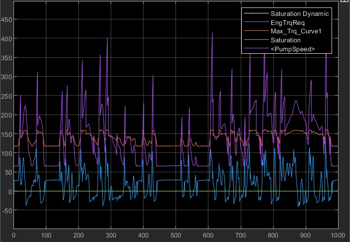
>The Engine speed gives the required torque from the controller,and is saturated between the Max torque curve and min torque curve and passes the engine torque to the Transmission block.

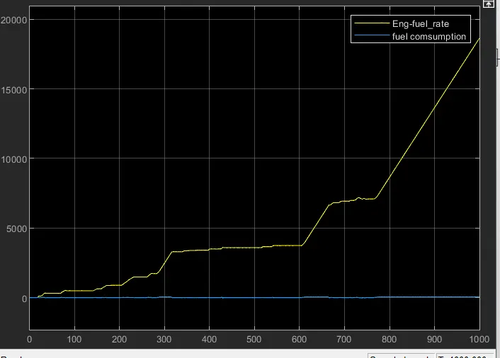
>The 2D look up table is used to claculate the fuel fow rate based on the engine trq,speed.The fuel flow rate is then integrated to find the fuel flow consumption.

>The estimated fuel flow rate ,fuel consumption,engien torque and engine speed are passed to the Matlab workspace using the workspace block.

Transmission Model:

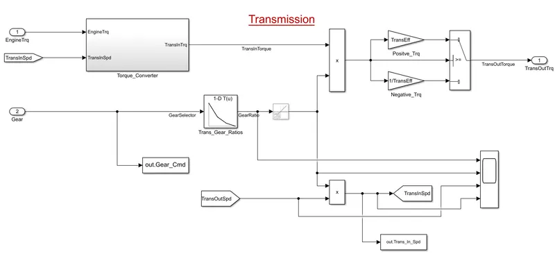
>Here the block contains another subsystem as Torque converter which convertes speed into the torque.

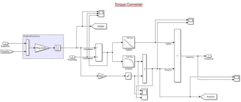
> The Engine Block is connected to the transmission via torque conerter.The output is given as signal to the differential.

Differential:

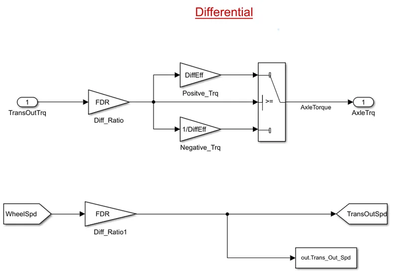
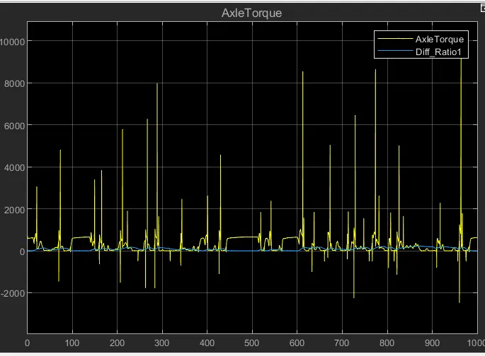
>From the transmission the signals is passes to the differential and here the output tirque is multiplied by the differential ratio and differential efficiency in this block after the torque is transmitted to the wheels as the axle torque.

Wheel Model:

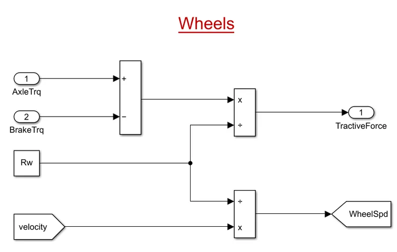
> Here the Brake Trq is subtracted from the Axle Trq and divides from the Rolling radius to determine the tractive froce.The wheel speed is calculated from the vehicle velocity and saved in the workspace.The output is taken as Tractive force.

Vehicle Dynamics:

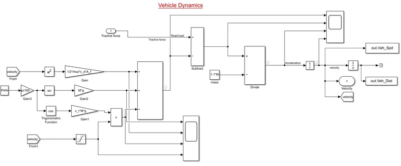
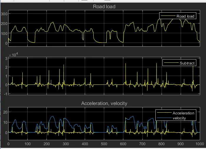
> The longitudinal dynamics of the vehcile along with the road load is represented in the vehicle dynamics block.The Tractive force and road load are used to calculated the vehicle velocity.

>Tractive force or tractive effort or traction is the force applied between the tire and road surface to move a car or any vehicle for that matter.

>The maximum permissible tractive force that can be applied to the wheels is governed by two things: the weight of the vehicle and the adhesion coefficient between the tire and the road surface.

>More the weight and the adhesion coefficient more amount of tractive force can be applied to the wheels without causing slips between the tires and road.

Formula Required:

Roadload=1/2*rhoa*c_d*A_f*(Vveh+V_h)^2+c_r*M*g*cosd(theta)+M*g*sind(theta)

Here,

rhoa=air density

Af=Frontal Area

Cd=Drag coefficient

Cr=rolling coefficient

M=mass of vehice

g=acceleration due to gravity

theta=slope angle

Output Plots:

> By running the model we get desired plots.Here these are combination of UDDS,HWFET files.

1.Driver cycle:

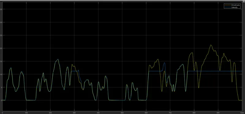
Actual velocity and Drive cycle

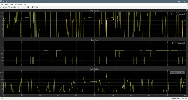
2.Control signal:

Engine Torque,Transmission Gear,Brake Torque:

3.Powertrain:

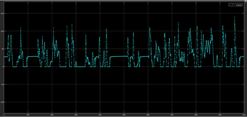
Engine:

Engine Torque:

Engine Fuel rate and fuel consumption:

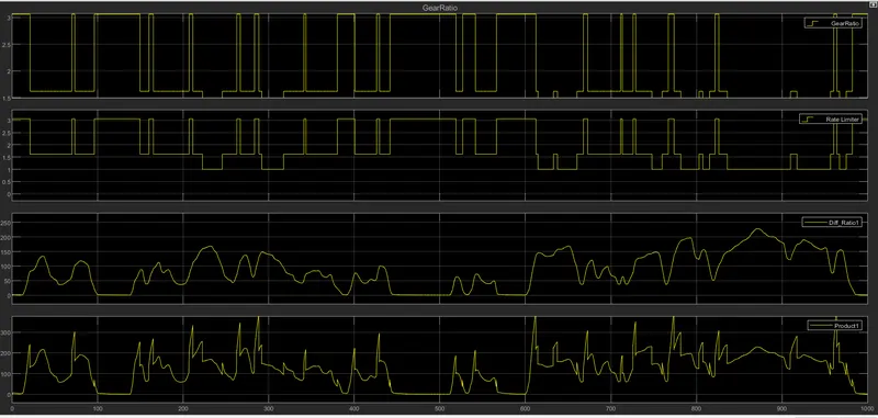
Transmission input and output speed,Gear ratio:

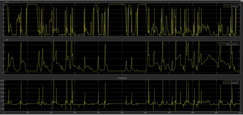
Torque Converter:

Differential Loads:

Axle torque and differential:

Wheel load:

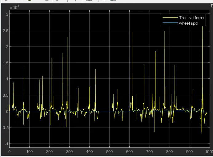
Tractive force,Road load Acceleration, velcoity:

Tractive force and wheel speed:

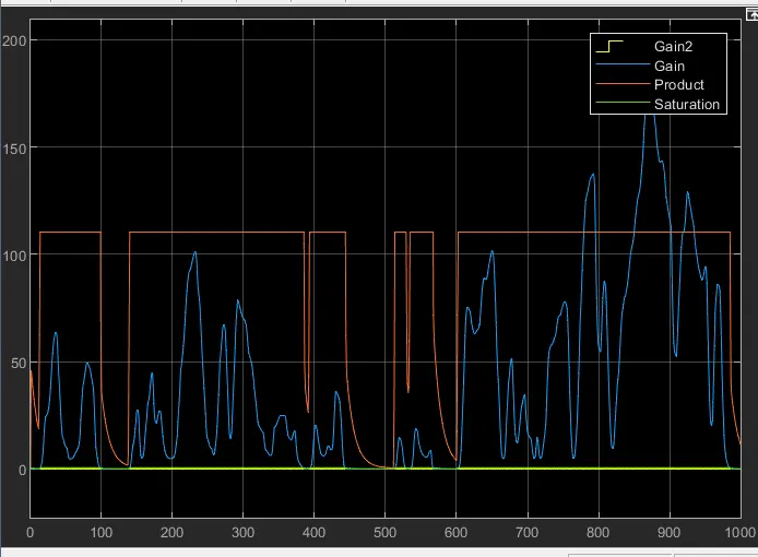
Vehicle Dynamics:

Post-Processing:

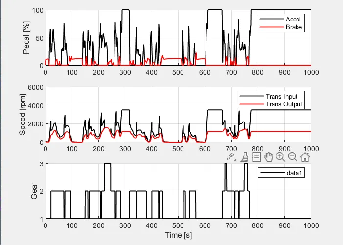
> A matlab script is created to analyse the data and to generated plots.Here we rename the variables loaded from the model,do some basic post-processing calculations and generates the results and plots.

%% Post-Processing File

% File for post-processing the Conventional vehicle simulation model data

%% Renaming variables

Time=out.tout;

Acc_Pdl = out.Acc_Pdl; % Accelerator pedal [%]

Brk_Pdl = out.Brk_Pdl; % Brake pedal [%]

Gear_Cmd = out.Gear_Cmd; % Transmission gear

Trans_In_Spd = out.Trans_In_Spd*30/pi; % Transmission input speed [rpm]

Trans_Out_Spd = out.Trans_Out_Spd*30/pi;% Transmission output speed [rpm]

Eng_Trq = out.Eng_Trq; % Engine brake torque [Nm]

Eng_Spd = out.Eng_Spd*30/pi; % Engine speed [rpm]

Eng_Fuel_Consump = out.Eng_Fuel_Consumption; % Engine fuel consumption [g]

Veh_Dist = out.Veh_Dist/1000; % Distance traveled by vehicle [km]

Veh_Spd = out.Veh_Spd*18/5; % Vehicle speed [kmph]

%% Data Analysis

Eng_Pwr = Eng_Spd*pi/30*Eng_Trq/1000; % Engine brake power [kW]

rho_petrol = 0.7197; % Density of petrol [kg/L]

kmpl = Veh_Dist(end)/(Eng_Fuel_Consump(end)/1000/rho_petrol); % Fuel economy [kmpl]

%% Plotting vehicle characteristics time trace

figure()

subplot(3,1,1)

hold on

grid on

plot(Time, Acc_Pdl, 'linewidth', 1, 'Color', 'black');

plot(Time, Brk_Pdl, 'linewidth', 1, 'Color', 'red');

ylabel('Pedal [%]')

xlim([0, Time(end)]);

legend('Accel','Brake');

subplot(3,1,2)

hold on

grid on

plot(Time, Trans_In_Spd, 'linewidth', 1, 'Color', 'black');

plot(Time, Trans_Out_Spd, 'linewidth', 1, 'Color', 'red');

ylabel('Speed [rpm]')

xlim([0, Time(end)]);

ylim([0, 6000]);

legend('Trans Input','Trans Output');

subplot(3,1,3)

hold on

grid on

plot(Time, Gear_Cmd, 'linewidth', 1, 'Color', 'black');

xlim([0, Time(end)]);

xlabel('Time [s]');

ylabel('Gear');

%% Plotting engine operating points on engine fuel map

figure('Name','Engine Operating Points');

hold on

grid on

title('Engine Operating Points','fontsize',12);

p1=plot(Eng_map_spd*30/pi,Eng_max_trq,'linewidth',2,'color','r');

p2=line([Eng_map_spd(end)*30/pi Eng_map_spd(end)*30/pi],[0 Eng_max_trq(end)]);

set(p2,'linewidth',1,'linestyle','--','color','k');

p3=line([Eng_map_spd(1)*30/pi Eng_map_spd(1)*30/pi],[0 Eng_max_trq(1)]);

set(p3,'linewidth',1,'linestyle','--','color','k');

[c,h] = contour(Eng_map_spd'*30/pi,Eng_map_trq,Eng_fuel_map');

clabel(c,h);

xlabel('Engine Speed [rpm]');

ylabel('Engine Torque [Nm]');

title('Engine Fuel Consumption Map [g/s]');

p4 = plot(Eng_Spd,Eng_Trq,'.','color','k');

legend([p1 p4],{'Max Curve','Operating Points'});

axis([Eng_map_spd(1)*30/pi Eng_map_spd(end)*30/pi 0 Eng_map_trq(end)]);

>After executing the file we get desired plots with combination of all given data

Output plot:

Project 1

Ship work like this
in your own course.

Talk to a career counsellor

Ship work like thisin your own course.

Talk to a career counsellor

Ship work like this
in your own course.