Project 1
Aim of the Project 1 is to do
- Tabulate the fuel economy numbers (kmpl) for UDDS and HWFET cycle. This forms the baseline numbers for comparing with the future hybrid version.
b. Plot the time trace for engine, transmission input, transmission output and wheel speed on one plot.
c. Plot engine torque, engine power, fuel rate and fuel consumption using subplots.
d. Plot accelerator and brake pedal, gear command, vehicle desired and actual speed, vehicle distance using subplots.
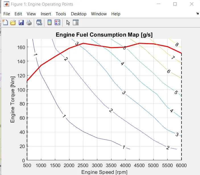
e. Plot the engine operating points on the engine fuel map.
f. Write down appropriate brief comments on each of these plots, describing the vehicle behavior throughout the drive cycle.
g. Generate the plots for both drive cycles.
First thing we are downloading the data files from the website.
Then we have open the matlab software to load the Project1_initfile.m file to get the matlab coding scrips for this projects.
In that codings we have to choose the which drive we neeed to do the calculation. In this thing we are going to select two drives UDDS and HWFET hybrid drives. After this now we are opening the simulink models in matlab to complete the vehicle dynamics model and engine models in powertrain drives sysyem.
simulink model
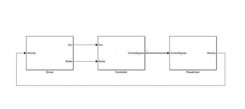
powertrain simulink models:
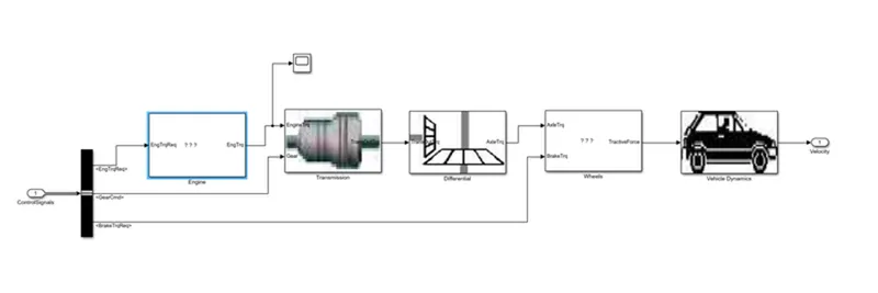
In this powertrain simulink models we are going to this vehicles dynamics models and engine drive models as shown below in the figure
Vehicle dynamics models:
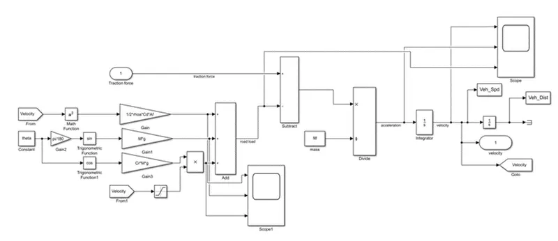
in this block diagram we were used different types of blocks and the matlab scrips were used for the simulation .
Here we were used this blocks like
1.constant blocks :- The Constant block generates a real or complex constant value signal. Use this block to provide a constant signal input. The block generates scalar, vector, or matrix output, depending on: The dimensionality of the Constant value parameter.
- SUM blocks:- The Sum block performs addition or subtraction on its inputs. The Add, Subtract, Sum of Elements, and Sum blocks are identical blocks. This block can add or subtract scalar, vector, or matrix inputs. It can also collapse the elements of a signal and perform a summation.
3.Subtract blocks
4.integrator blocks :- The Integrator block accepts and outputs signals of type double on its data ports. The external reset port accepts signals of type double or Boolean .
5.gain blocks :- The Gain block multiplies or ADD the input by a constant value (gain). The input and the gain can each be a scalar, vector, or matrix. You specify the value of gain in the Gain parameter. The Multiplication parameter lets you specify element-wise or matrix multiplication.
6.goto and from blocks:- The Goto block passes its input to its corresponding From blocks. The input can be a real- or complex-valued signal or vector of any data type. From and Goto blocks allow you to pass a signal from one block to another without actually connecting them.
7.triginomentary blocks:- The Trigonometric Function block performs numerous common trigonometric functions. You can select one of these functions from the Function list: sin , cos , tan , asin , acos , atan , atan2 , sinh , cosh , and tanh . The block output is the result of the operation of the function on the input or inputs.
8.scope blocks :- The Scope block displays its input with respect to simulation time. The Scope block can have multiple axes (one per port); all axes have a common time range with independent y-axes. The Scope allows you to adjust the amount of time and the range of input values displayed.
- to work space blocks:- The To Workspace block writes input signal data to a workspace. During simulation, the block writes data to an internal buffer. When you pause the simulation or the simulation completes, that data is written to the workspace.
Before we were discussed about the what qre the blocks were used in the block diagram and ther uses. Now we are going to see the calculation and how the the blocks is connected each other.
First from the traction force input blocks is connected to the sum blocks and in the sum blocks the traction force and road load is subtracted. for the road load calculation this formula were used as given below
fload = 1/2*rhoa*cd*af*(Vveh+Vwind)^2+cr*m*g*cosd(theta)+m*g*sind(theta) % road load in N
pload = fload*Vveh/1000 % road load power in kw
in simulink were are going to add this formula by this methosd asshown below
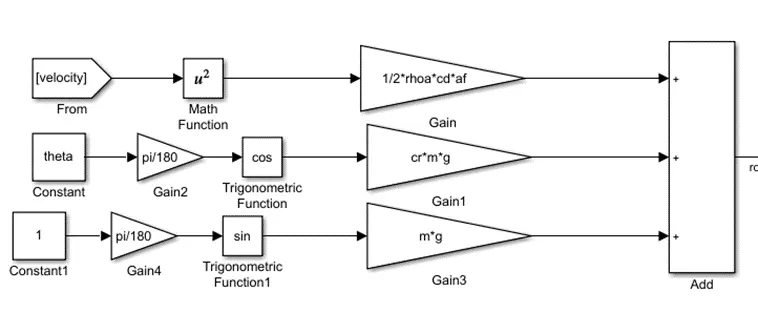
in this block diagram the velocity in from block signal were getting from the goto block and its squarerooted by the math functions and to the gain blocks the signal is connected to thee Add sum blocks to add all the integers
in the second line the constant blocks were used to represent he theta value and then the theata is converted to the degree by this formula pi/180 and connected to the trignometric function blocks and then multiply with gain blocks with cr*m*g formula directly imported from the matlab coding and then add
same as mentioned for this function the formula 3*g ics calculated and ouput added to add sum blocks .
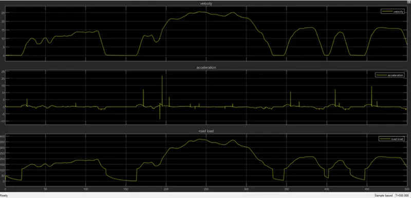
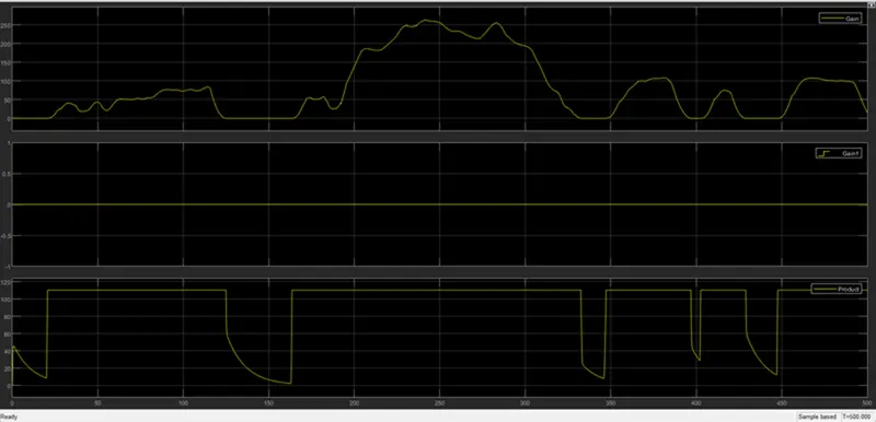
These three integers were added in the ADD sum block as a roadload value. then road value is connected to subtact sum block to do calculated the tractionforce minus road load then the signal is connected to divide sum block . in this it gets divided by mass to the acceleration value. then it connected with the integrator block to get the velocity . Then the roadload , acceleration and the velocity is connected to the scope blocks to get graphicall repersentation. then here we are usind the terminator blocks to stop the outputs values.
outputs of vehicle dynamics:
Engine drive models:
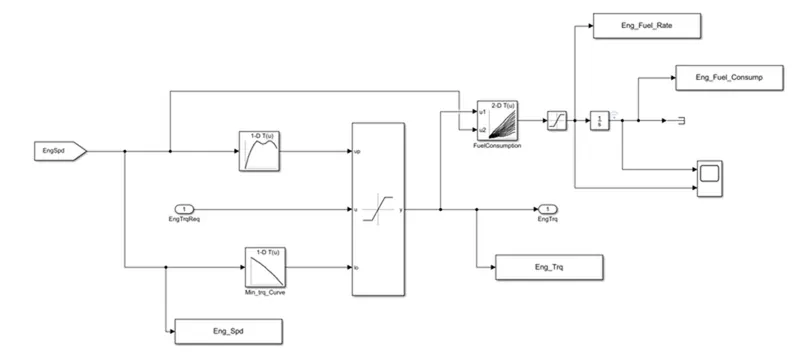
in this engine drive models we are using different types of blocks
1.integrator blocks :- The Integrator block accepts and outputs signals of type double on its data ports. The external reset port accepts signals of type double or Boolean .
2.goto and from blocks:- The Goto block passes its input to its corresponding From blocks. The input can be a real- or complex-valued signal or vector of any data type. From and Goto blocks allow you to pass a signal from one block to another without actually connecting them.
3.to work space blocks:- The To Workspace block writes input signal data to a workspace. During simulation, the block writes data to an internal buffer. When you pause the simulation or the simulation completes, that data is written to the workspace.
4..scope blocks :- The Scope block displays its input with respect to simulation time. The Scope block can have multiple axes (one per port); all axes have a common time range with independent y-axes. The Scope allows you to adjust the amount of time and the range of input values displayed.
5.1-D Lookup table generates an output signal by interpolating based on a given data set and input value. The Input values x property must be a strictly increasing or decreasing array.
- 2-D lookup table blocks:-The Lookup Table (2D) block computes an approximation of output value with given values of two (2D) inputs and outputs using the specified lookup method.
7.Saturation Dynamic blocks:- The Saturation block produces an output signal that is the value of the input signal bounded to the upper and lower saturation values. The upper and lower limits are specified by the parameters Upper limit and Lower limit.
- Saturation Blocks:- The Saturation block imposes upper and lower bounds on a signal. When the input signal is within the range specified by the Lower limit and Upper limit parameters, the input signal passes through unchanged.
in this simulink models we getting singnal from from block. engine from blocks is connected with the maximum and minimum 1-d lookup block. this both blocks were connected to the saturation dynamic models.then the signals is passed to engine trq here we have coonected the to workspace blocks get simulink values in the matlab workspace. Engspeed blocks is connected with the 2-d lookup table the from the 2-d lookup table the outputs signals is connected with the saturation block and intergrator blocks and this block is connected with the scope block to get outputs. then also coonected with the to workspace block to import the values in matlab workspace. In this engine sub system blocks engsped,engtrq, engine fuel rate and engone fuel consumption to workspace blocks is connected to get the values in the matlab workspace for the plotting the graphs of the engine.
scope of engine subsystem:-
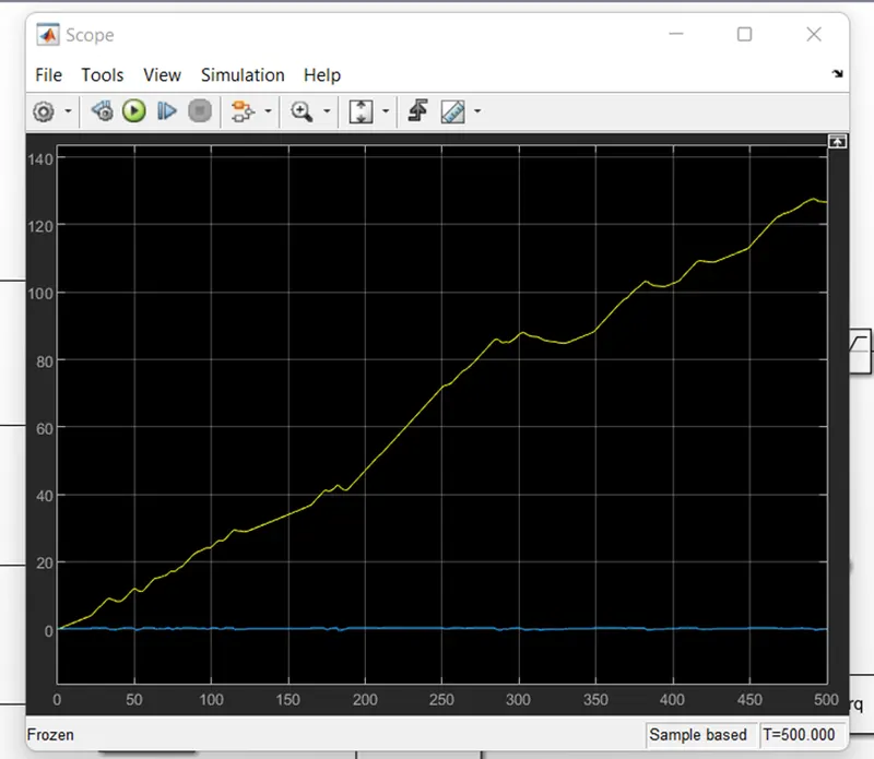
Engine torque otputs from the scope blocks:
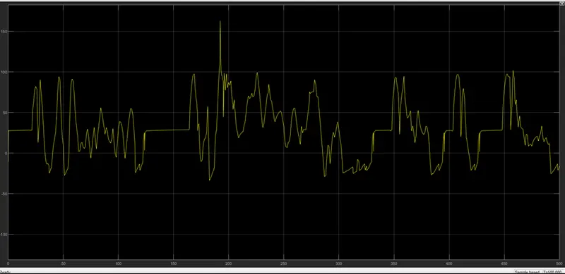
matlab codings for uuds cycle:
%% Vehicle Parameters
M = 1500; % Vehicle weight [kg]
Cr = 0.015; % Rolling resistance coefficient
Rw = 0.35; % Rolling radius [m]
Cd = 0.33; % Drag coefficient
Af = 2; % Frontal area [m2]
rhoa = 1.225; % Air density [kg/m3]
Vwind = 0; % Wind velocity [kmph]
g = 9.81; % Gravitational acceleration [m/s2]
theta = 0; % Slope [deg]
myu_road_tire = 1; % Coefficient of friction between tire - road interface
%% Powertrain Parameters
FDR = 3.73; % Final Drive Ratio / Diff Ratio
DiffEff = 0.99; % Differential efficiency (assumed independent of operating conditions)
NumGear = 4; % Number of gears in transmission
TransGear = [1:NumGear]; % Transmission Gears
TransRatio = [3.06, 1.62, 1, 0.7]; % Corresponding Transmission ratios
TransEff = 0.90; % Transmission efficiency (assumed independent of operating conditions)
TC_SR = [0, .5, .6, .7, .8, .87, .92, .94, .96, .97, 1]; % Torque Converter Speed Ratio (Matlab default) -> TurbSpd/PumpSpd
TC_TR = [2.232, 1.5462, 1.4058, 1.2746, 1.1528, 1.0732, 1.0192, 1, 1, 1, 1]; % Torque Converter Torque Ratio (Matlab default) -> TurbTrq/PumpTrq
TC_Cf = 1e-4 * [.72558, .66322, .63463, .59042, .51331, .4144, .29287, .22444, .12186, .04386, 0]; % Torque Converter Capacity Factor (Matlab default) -> PumpTrq/PumpSpd^2 [Nm/rpm^2]
load Vehicle_Data/Engine_data_1_9L_Saturn_95kW
load Vehicle_Data/Trans_Shift_map
%% Driver Parameters
Kp = 10; % P gain for driver PI model
Ki = 1; % I gain for driver PI model
Drive_Cycle_Select = 1; % Drive cycle selection
% Drive cycle values in m/s
if Drive_Cycle_Select == 1
load DriveCycles/UDDS;
elseif Drive_Cycle_Select == 2
load DriveCycles/HWFET;
elseif Drive_Cycle_Select == 3
load DriveCycles/FTP;
elseif Drive_Cycle_Select == 4
load DriveCycles/US06;
elseif Drive_Cycle_Select == 5
load DriveCycles/NEDC;
elseif Drive_Cycle_Select == 6
load DriveCycles/WLTP;
end
time_end = cyc_time(end);
vel_end = cyc_vel(end);
Time = out.tout;
Acc_Pdl = out.Acc_Pdl; % Accelerator pedal [%]
Brk_Pdl = out.Brk_Pdl; % Brake pedal [%]
Gear_Cmd = out.Gear_Cmd; % Transmission gear
Trans_In_Spd = out.Trans_In_Spd*30/pi; % Transmission input speed [rpm]
Trans_Out_Spd = out.Trans_Out_Spd*30/pi;% Transmission output speed [rpm]
Eng_Trq = out.Eng_Trq; % Engine brake torque [Nm]
Eng_Spd = out.Eng_Spd*30/pi; % Engine speed [rpm]
Eng_Fuel_Consump = out.Eng_Fuel_Consumption; % Engine fuel consumption [g]
Veh_Dist = out.Veh_Dist/1000; % Distance traveled by vehicle [km]
Veh_Spd = out.Veh_Spd*18/5; % Vehicle speed [kmph]
%% Data Analysis
Eng_Pwr = Eng_Spd*pi/30*Eng_Trq/1000; % Engine brake power [kW]
rho_petrol = 0.7197; % Density of petrol [kg/L]
%kmpl = (Veh_Dist(end)/(Eng_Fuel_Consump(end)/1000/rho_petrol)); % Fuel economy [kmpl]
%% Plotting vehicle characteristics time trace
figure(3)
subplot(3,1,1)
hold on
grid on
plot(Time, Acc_Pdl, 'linewidth', 1, 'Color', 'black');
plot(Time, Brk_Pdl, 'linewidth', 1, 'Color', 'red');
ylabel('Pedal [%]')
xlim([0, Time(end)]);
legend('Accel','Brake');
subplot(3,1,2)
hold on
grid on
plot(Time, Trans_In_Spd, 'linewidth', 1, 'Color', 'black');
plot(Time, Trans_Out_Spd, 'linewidth', 1, 'Color', 'red');
ylabel('Speed [rpm]')
xlim([0, Time(end)]);
ylim([0, 6000]);
legend('Trans Input','Trans Output');
subplot(3,1,3)
hold on
grid on
plot(Time, Gear_Cmd, 'linewidth', 1, 'Color', 'black');
xlim([0, Time(end)]);
xlabel('Time [s]');
ylabel('Gear');
%% Plotting engine operating points on engine fuel map
figure('Name','Engine Operating Points');
hold on
grid on
title('Engine Operating Points','fontsize',12);
p1=plot(Eng_map_spd*30/pi,Eng_max_trq,'linewidth',2,'color','r');
p2=line([Eng_map_spd(end)*30/pi Eng_map_spd(end)*30/pi],[0 Eng_max_trq(end)]);
set(p2,'linewidth',1,'linestyle','--','color','k');
p3=line([Eng_map_spd(1)*30/pi Eng_map_spd(1)*30/pi],[0 Eng_max_trq(1)]);
set(p3,'linewidth',1,'linestyle','--','color','k');
[c,h] = contour(Eng_map_spd'*30/pi,Eng_map_trq,Eng_fuel_map');
clabel(c,h);
xlabel('Engine Speed [rpm]');
ylabel('Engine Torque [Nm]');
title('Engine Fuel Consumption Map [g/s]');
p4 = plot(Eng_Spd,Eng_Trq,'.','color','k');
legend([p1 p4],{'Max Curve','Operating Points'});
axis([Eng_map_spd(1)*30/pi Eng_map_spd(end)*30/pi 0 Eng_map_trq(end)]);
plotting the graphs
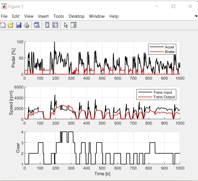
engine fuel consumption fuel rate map
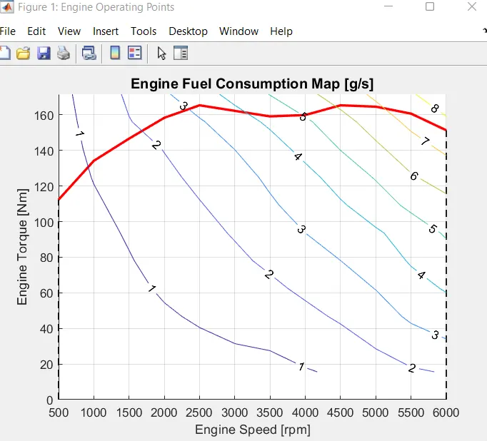
codings for hwfet cycle:
%% Vehicle Parameters
M = 1500; % Vehicle weight [kg]
Cr = 0.015; % Rolling resistance coefficient
Rw = 0.35; % Rolling radius [m]
Cd = 0.33; % Drag coefficient
Af = 2; % Frontal area [m2]
rhoa = 1.225; % Air density [kg/m3]
Vwind = 0; % Wind velocity [kmph]
g = 9.81; % Gravitational acceleration [m/s2]
theta = 0; % Slope [deg]
myu_road_tire = 1; % Coefficient of friction between tire - road interface
%% Powertrain Parameters
FDR = 3.73; % Final Drive Ratio / Diff Ratio
DiffEff = 0.99; % Differential efficiency (assumed independent of operating conditions)
NumGear = 4; % Number of gears in transmission
TransGear = [1:NumGear]; % Transmission Gears
TransRatio = [3.06, 1.62, 1, 0.7]; % Corresponding Transmission ratios
TransEff = 0.90; % Transmission efficiency (assumed independent of operating conditions)
TC_SR = [0, .5, .6, .7, .8, .87, .92, .94, .96, .97, 1]; % Torque Converter Speed Ratio (Matlab default) -> TurbSpd/PumpSpd
TC_TR = [2.232, 1.5462, 1.4058, 1.2746, 1.1528, 1.0732, 1.0192, 1, 1, 1, 1]; % Torque Converter Torque Ratio (Matlab default) -> TurbTrq/PumpTrq
TC_Cf = 1e-4 * [.72558, .66322, .63463, .59042, .51331, .4144, .29287, .22444, .12186, .04386, 0]; % Torque Converter Capacity Factor (Matlab default) -> PumpTrq/PumpSpd^2 [Nm/rpm^2]
load Vehicle_Data/Engine_data_1_9L_Saturn_95kW
load Vehicle_Data/Trans_Shift_map
%% Driver Parameters
Kp = 10; % P gain for driver PI model
Ki = 1; % I gain for driver PI model
Drive_Cycle_Select = 1; % Drive cycle selection
% Drive cycle values in m/s
if Drive_Cycle_Select == 1
load DriveCycles/UDDS;
elseif Drive_Cycle_Select == 2
load DriveCycles/HWFET;
%elseif Drive_Cycle_Select == 3
%load DriveCycles/FTP;
%elseif Drive_Cycle_Select == 4
%load DriveCycles/US06;
%elseif Drive_Cycle_Select == 5
%load DriveCycles/NEDC;
%elseif Drive_Cycle_Select == 6
%load DriveCycles/WLTP;
end
time_end = cyc_time(end);
vel_end = cyc_vel(end);
Time = out.tout;
Acc_Pdl = out.Acc_Pdl; % Accelerator pedal [%]
Brk_Pdl = out.Brk_Pdl; % Brake pedal [%]
Gear_Cmd = out.Gear_Cmd; % Transmission gear
Trans_In_Spd = out.Trans_In_Spd*30/pi; % Transmission input speed [rpm]
Trans_Out_Spd = out.Trans_Out_Spd*30/pi;% Transmission output speed [rpm]
Eng_Trq = out.Eng_Trq; % Engine brake torque [Nm]
Eng_Spd = out.Eng_Spd*30/pi; % Engine speed [rpm]
Eng_Fuel_Consump = out.Eng_Fuel_Consumption; % Engine fuel consumption [g]
Veh_Dist = out.Veh_Dist/1000; % Distance traveled by vehicle [km]
Veh_Spd = out.Veh_Spd*18/5; % Vehicle speed [kmph]
%% Data Analysis
Eng_Pwr = Eng_Spd*pi/30*Eng_Trq/1000; % Engine brake power [kW]
rho_petrol = 0.7197; % Density of petrol [kg/L]
%kmpl = (Veh_Dist(end)/(Eng_Fuel_Consump(end)/1000/rho_petrol)); % Fuel economy [kmpl]
%% Plotting vehicle characteristics time trace
figure(3)
subplot(3,1,1)
hold on
grid on
plot(Time, Acc_Pdl, 'linewidth', 1, 'Color', 'black');
plot(Time, Brk_Pdl, 'linewidth', 1, 'Color', 'red');
ylabel('Pedal [%]')
xlim([0, Time(end)]);
legend('Accel','Brake');
subplot(3,1,2)
hold on
grid on
plot(Time, Trans_In_Spd, 'linewidth', 1, 'Color', 'black');
plot(Time, Trans_Out_Spd, 'linewidth', 1, 'Color', 'red');
ylabel('Speed [rpm]')
xlim([0, Time(end)]);
ylim([0, 6000]);
legend('Trans Input','Trans Output');
subplot(3,1,3)
hold on
grid on
plot(Time, Gear_Cmd, 'linewidth', 1, 'Color', 'black');
xlim([0, Time(end)]);
xlabel('Time [s]');
ylabel('Gear');
%% Plotting engine operating points on engine fuel map
figure('Name','Engine Operating Points');
hold on
grid on
title('Engine Operating Points','fontsize',12);
p1=plot(Eng_map_spd*30/pi,Eng_max_trq,'linewidth',2,'color','r');
p2=line([Eng_map_spd(end)*30/pi Eng_map_spd(end)*30/pi],[0 Eng_max_trq(end)]);
set(p2,'linewidth',1,'linestyle','--','color','k');
p3=line([Eng_map_spd(1)*30/pi Eng_map_spd(1)*30/pi],[0 Eng_max_trq(1)]);
set(p3,'linewidth',1,'linestyle','--','color','k');
[c,h] = contour(Eng_map_spd'*30/pi,Eng_map_trq,Eng_fuel_map');
clabel(c,h);
xlabel('Engine Speed [rpm]');
ylabel('Engine Torque [Nm]');
title('Engine Fuel Consumption Map [g/s]');
p4 = plot(Eng_Spd,Eng_Trq,'.','color','k');
legend([p1 p4],{'Max Curve','Operating Points'});
axis([Eng_map_spd(1)*30/pi Eng_map_spd(end)*30/pi 0 Eng_map_trq(end)]);
graphs for hwfet cyclwes:
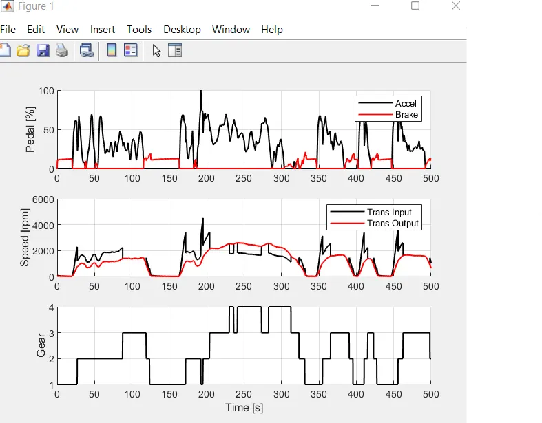
in graphs we have shown the graph for time vs gear, speed vs time and acceleration vs brake
plot engine torque, engine power, fuel rate and fuel consumption using subplots.