Week 4.1 - Genetic Algorithm

Functions for the ga stalagmite function

function [f] = stalagmite(input_vector)
x = input_vector(1);
y = input_vector(2);
f1 = (sin(5.1*pi*x + 0.5)).^6;
f2 = (sin(5.1*pi*y + 0.5)).^6;
f3 = exp((-4.*log(2)*(x-0.0667).^2)/(0.64));
f4 = exp((-4.*log(2)*(y-0.0667).^2)/(0.64));
f = -(f1*f2*f3*f4);
end

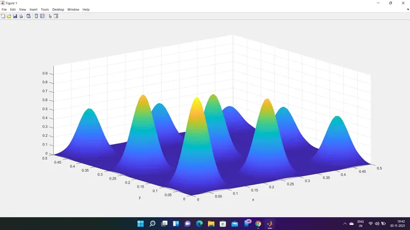
creating the surfaceplot as stalagemite function

clear all
close all
clc

%providing the search space forthe function
x=linspace(0,0.5,100);
y=linspace(0,0.5,100);
[xx,yy]=meshgrid(x,y);

num_cases=50;
%creating the surfaceplot as stalagemite function

for i=1:length(x)
for j=1:length(y)
input_vector(1)=xx(i,j);
input_vector(2)=yy(i,j);
f(i,j)=stalagmite(input_vector);
end
end
surfc(xx,yy,-f);
xlabel('x')
ylabel('y')
shading interp

[x,fval] = ga(@stalagmite,2)

main codings for all the genatic algorthim

1.statistical behaviour for unbounded

2.statistical behaviour for bounded

3. no of population by increasing the population by options.

codings

clear all
close all
clc

%providing the search space forthe function
x=linspace(0,0.6,300);
y=linspace(0,0.6,300);
[xx,yy]=meshgrid(x,y);

num_cases=50;
%creating the surfaceplot as stalagemite function

for i=1:length(x)
for j=1:length(y)
input_vector(1)=xx(i,j);
input_vector(2)=yy(i,j);
f(i,j)=stalagmite(input_vector);
end
end

% statistical behaviour for unbounded
num_cases = 50; % GA runs for 50 itreations
tic % study time count starts
for i=1:num_cases
[input,fopt(i)]=ga(@stalagmite,2);
xopt(i)=input(1);
yopt(j)=input(2);
optf(i)=-fopt(i); %ga gives the minima value. inverse f_opt is taken as a maxima value.
end
study_time = toc % study time count ends
%plotting the graph
figure(1)
subplot(2,1,1)
surfc(xx,yy,-f) % generation of stalagmite function
hold on
shading interp % to bring the smooth curve without mesh lines.
%plot3(xopt,yopt,-fopt,'marker','g','markersize',3,'markerfacecolor','r')
xlabel('x');
ylabel('y');
grid on
title('unbounded inputs')
subplot(2,1,2)
plot(-fopt)% plot of optimum function for every iterations
xlabel('number of iterations-->')
ylabel('function min-->')

% statistical behaviour for bounded
num_cases = 60 % GA runs for 60 itreations
tic % study time count starts
for j=1:num_cases
[input,fopt(j)]=ga(@stalagmite,2,[],[],[],[],[0;0],[1,1]);
xopt(j)=input(1);
yopt(j)=input(2);
optf(j)=-fopt(j); %ga gives the minima value. inverse f_opt is taken as a maxima value.
end
study_time = toc % study time count ends
%plotting the graph
figure(2)
subplot(2,1,1)
surfc(xx,yy,-f) % generation of stalagmite function
hold on
shading interp % to bring the smooth curve without mesh lines.
%plot3(xopt,yopt,-fopt,'marker','g','markersize',3,'markerfacecolor','r')
xlabel('x');
ylabel('y');
grid on
title('Bounded inputs')
subplot(2,1,2)
plot(-fopt)% plot of optimum function for every iterations
xlabel('number of iterations-->')
ylabel('function min-->')

% modifying the number of population
num_cases = 30; % GA runs for 30 itreations
options=optimoptions('ga','populationsize',300)
tic % study time count starts
for k=1:num_cases
[input,fopt(k)]=ga(@stalagmite,2,[],[],[],[],[0;0],[1;1],[],[],options);
xopt(k)=input(1);
yopt(k)=input(2);
optf(k)=-fopt(k); %ga gives the minima value. inverse f_opt is taken as a maxima value.
end
study_time = toc % study time count ends
%plotting the graph
figure(3)
subplot(2,1,1)
surfc(xx,yy,-f) % generation of stalagmite function
hold on
shading interp % to bring the smooth curve without mesh lines.
%plot3(xopt,yopt,-fopt,'marker','g','markersize',3,'markerfacecolor','r')
xlabel('x');
ylabel('y');
grid on
title('Number of populations inputs')
subplot(2,1,2)
plot(-fopt)% plot of optimum function for every iterations
xlabel('number of iterations-->')
ylabel('function min-->')