Project 1
Aim:
To Design and to the development of a forward energy-based fuel consumption model of a conventional vehicle using MATLAB and SIMULINK Software
Procedure:
To determine the given parameters and scripts develop the MATLAB code and SIMULINK blocks for the given 1.9L Engine and a 4-speed automatic transmission, there are 6 different Drive Cycles has been given, we use UDDS and HWFET Drive Cycles for this project, the procedure as follows
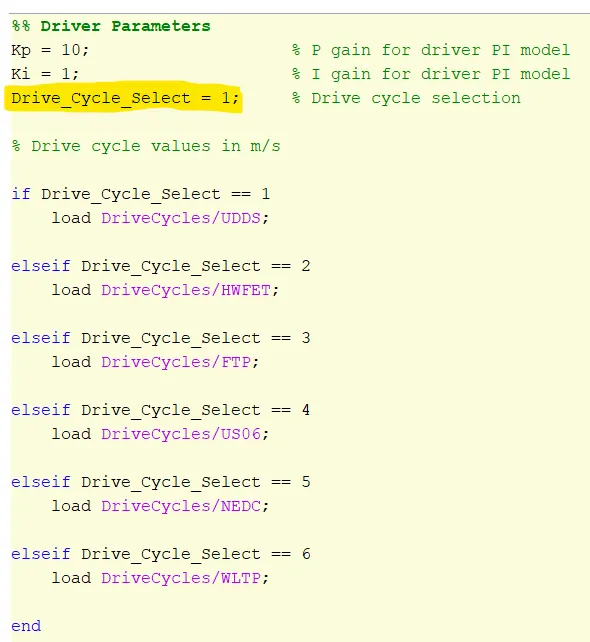
Load the “Project1_InitFile.m” file in the MATLAB Software and Run the code, in the code there are different drive cycles, here we take UDDS into consideration and the related parameters are been coded with the required values, for different drive cycles different values has been loaded as shown below with Drive Cycle 1 is UDDS and Drive Cycle 2 is HWFET.
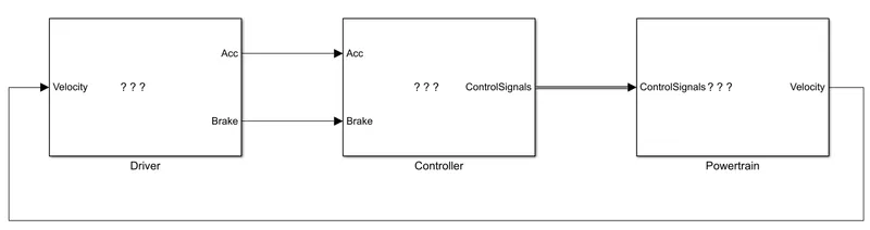
Once the Initial file has been loaded and Run Successfully, SIMULINK file "Project1_VehicleModel.slx" should be loaded in the SIMULINK Software, it contains Vehicle model with Driver, Controller and Powertrain as the Main block system.
Inside the Driver Block, the Subsystem blocks has been created with desired parameters as below, 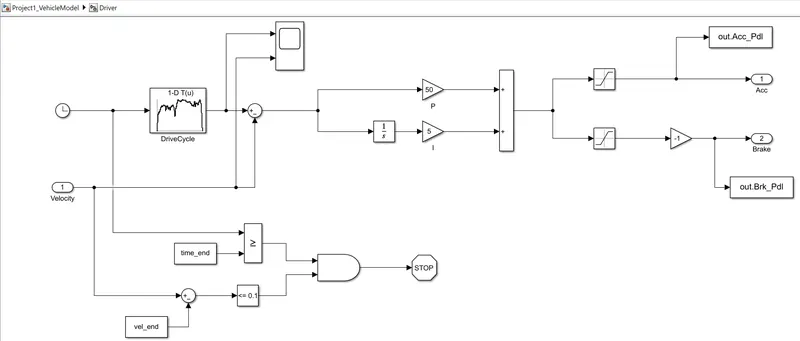
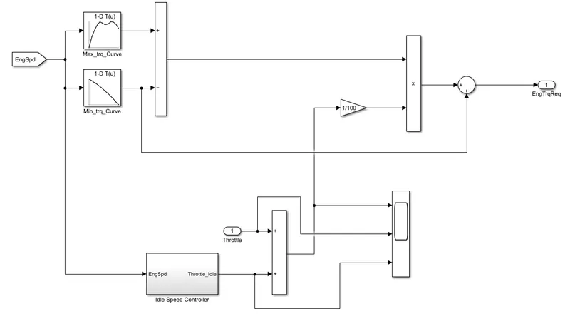
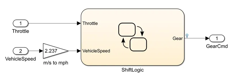
In the Controller Block, the Subsystem blocks Engine Control Unit, Transmission Control Unit and Brake Control Unit has been created with each subsystem blocks has created with different parameters as below,
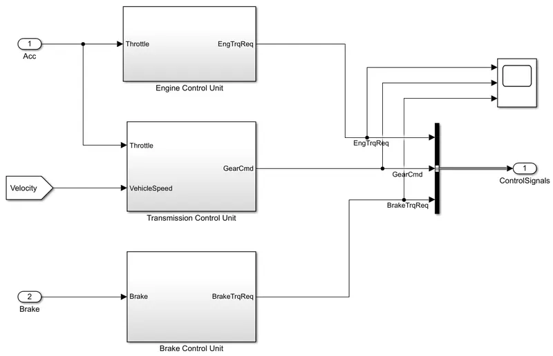
Engine Control Unit:
Transmission Control Unit:
Brake Control Unit:
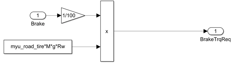
The above blocks are created inside the Controller Unit Block, this blocks are already created in the file itself.
In the Powertrain Block we have Engine, Transmission, Differential, Wheels, Vehicle Dynamics block as above the Transmission, Differential, Wheels blocks are already been created in the file itself.
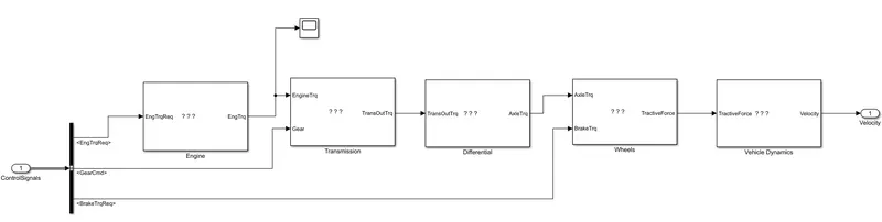
Engine Block:
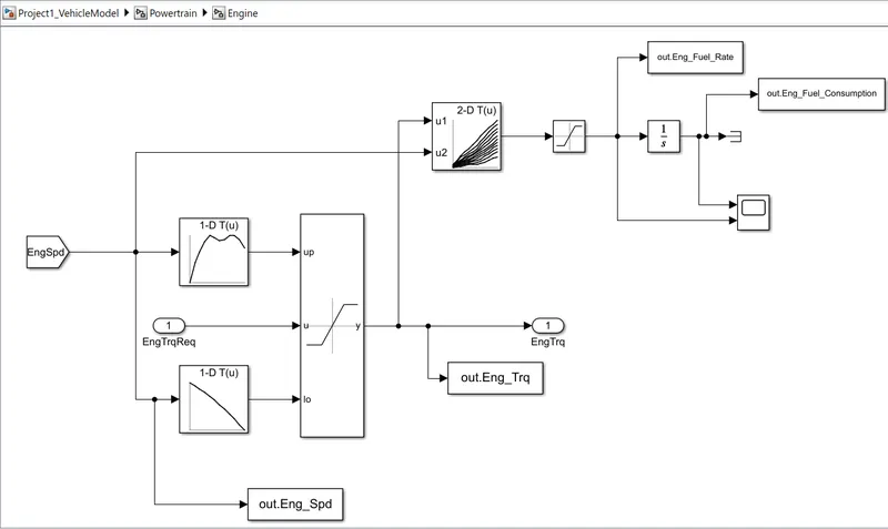
The Engine block is loaded with the Engine Speed, Torque and Fuel flow rate and Fuel Consumption, Lookup Table Block has been created to load the datas of Engine Fuel Map, Engine Map Speed, Engine map Torque has been loaded from the Simulated MATLAB file where the datas in the results has been used. Engine torque has been kept as monitoring the torque value is positive or negative.
Vehicle Dynamics:
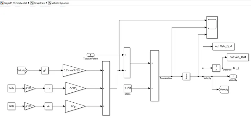
The Vehicle Dynamics block has been build with the equation of Mass time Acceleration is the Tractive force, to get the velocity we have to divide the Tractive force with the Mass as shown in below image, the blocks are created accordingly with intregator, Gain block, Trignomentry block, Addition block, Goto block.

Once the Blocks are created, To Workspace blocks should be created so that once the SIMULINK is simulated the resultant values will be transferred to the MATLAB Workspace and the plotting will be gained. This To Workspace blocks are connected to the Engine Fuel Rate, Engine Fuel Consumption, Engine Speed, Engine Torque, Vehicle Speed and Vehicle Torque.
Now the SIMULINK Model is simulated to see the resultant of the Vehicle Dynamics which can be seen through scope for reference.
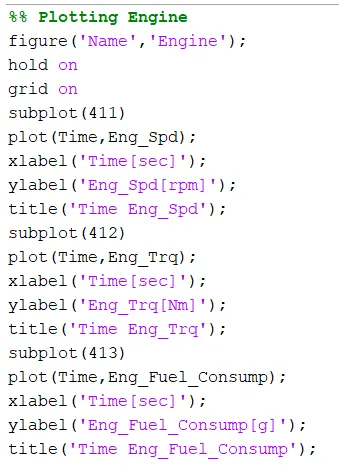
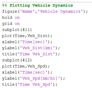
Then Load the Processing file of MATLAB in the attached file, edit the model of Data Analysis as the dot product with the 'pi' and for the Eng_Trq since Eng_Spd is not a single value it has multiple values.

Now, plotting the graph of Engine with Engine Speed, Torque and Fuel Consumption and Vehicle with Vehicle Distance and Speed as shown below,
Now, check the OUT result in the workspace whether the Eng_Spd, Eng_Trq, Eng_Fuel_Consumption, Veh_Spd, Veh_Distance has been reflected in the Workspace of MATLAB.
The process file is made to RUN, with the UDDS file data and the results are as below,
For UDDS File:
Figure1:
In the Figure 1 the result of Acceleration, Speed and Gear with respect to time has been shown in below graph, here the acceleration is black lines and red ines are brakes where there is always and increase and decrease according to the road condition, traffic, etc.. and also brakes are applied accordingly. The second subplot indicates the Speed of the vehicle and the third plot indicates the wich gear the Vehicle is operated
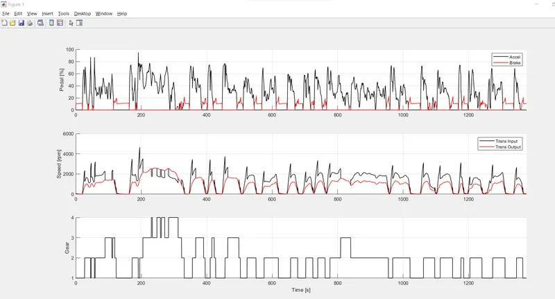
Figure2:
In the Figure 2 the Contour plot of Engine Fuel Consumption is obtained with respect to Engine Torque and Engine Speed, the dot points shows the Vehicle Opersating points where the Max Curve is given in the red line.
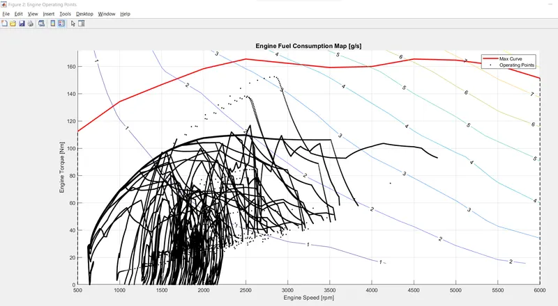
Figure3:
In Figure 3 Engine details are been obtained as Engine Speed , Torque, Fuel Consumption has been obtained with respect to the Time.
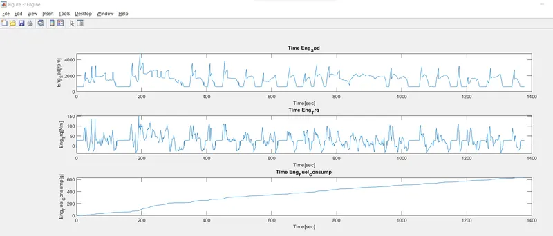
Figure4:
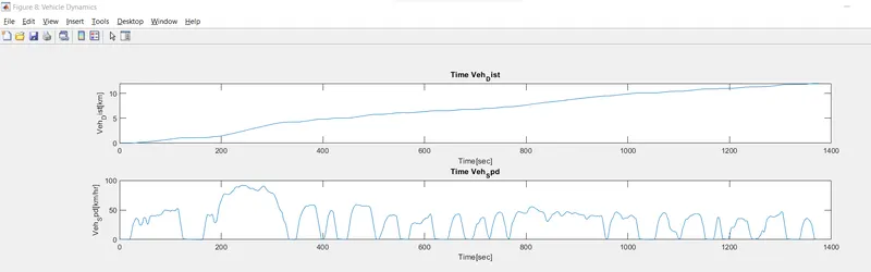
In Figure 4 Vehicle Dynamics details are been obtained as Vehicle Speed, Vehicle Distance is obtained with respect to the Time.
Workspace Result of UDDS:
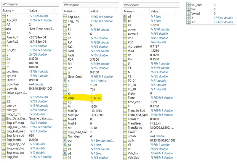
The file UDDS data has the kmpl of 13.6312 which is highlightedin the below image.
For HWFET File:
Figure1:
In the Figure 1 the result of Acceleration, Speed and Gear with respect to time has been shown in below graph, here the acceleration is black lines and red ines are brakes where there is always and increase and decrease according to the road condition, traffic, etc.. and also brakes are applied accordingly. The second subplot indicates the Speed of the vehicle and the third plot indicates the wich gear the Vehicle is operated
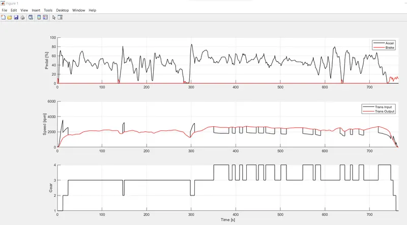
Figure2:
In the Figure 2 the Contour plot of Engine Fuel Consumption is obtained with respect to Engine Torque and Engine Speed, the dot points shows the Vehicle Opersating points where the Max Curve is given in the red line.
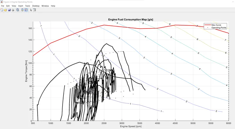
Figure3:
In Figure 3 Engine details are been obtained as Engine Speed, Torque, Fuel Consumption has been obtained with respect to the Time.
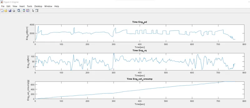
Figure4:
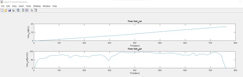
In Figure 4 Vehicle Dynamics details are been obtained as Vehicle Speed, Vehicle Distance is obtained with respect to the Time.
Workspace Result of UDDS:
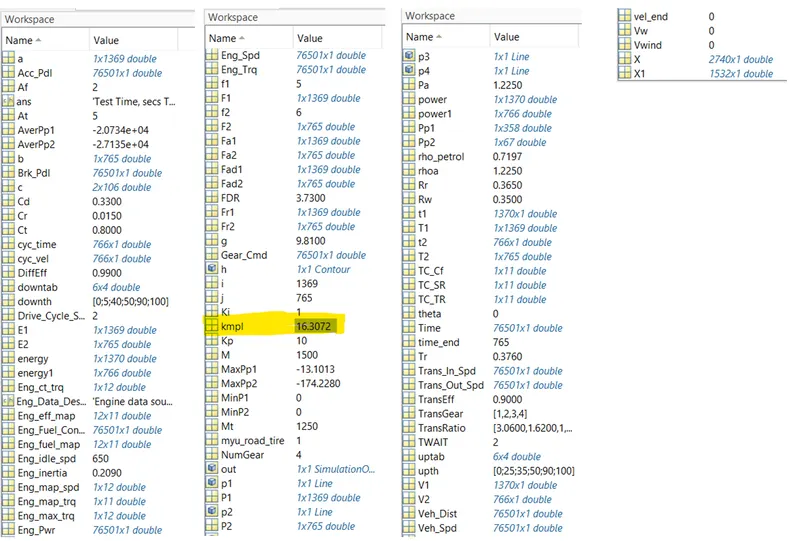
The file UDDS data has the kmpl of 16.3072 which is highlightedin the below image.
Result:
In the above procedure and the results we can see the HWFET cycle gives 16.3072kmpl and UDDS has 13.6312kmpl as a conclusion the HWFET cycle vehicle is more Efficient when compared to the UDDS cycle.