Week 4.1 - Genetic Algorithm

Aim:

To creat a code in MATLAB to optimise the stalagmite function and find the global maxima of the function, explain the concept of Genetic Algorithm and the syntax for GA in MATLAB.

Procedure:

Objective:

• Understand Genetic Algorithm, Optimization, Syntax of Genetic Algorithm
• To derive Stalagmite expression using given data
• Plot the graph for stalagmite function, unbounded or unconstrained condition & for constrained condition

Understanding Genetic Algorithm:

• Genetic algorithm first discovered by John Holland, it is based on random sampling in which the random input parameters are given to calculate the function based on the inputs provided
• It is based on Genetics and Natural Selection.
• GA is used to solve the optimal solutions to the problem, which is difficult to solve in real time.
• GA in MATLAB always minimize the function

Optimization:

• Optimization refers to find the values of inputs to get the best output.
• Based on the different input parameters provided it can be analyse the minimize or maximize the particular function, it is executed iteratively untill the optimum solution is obtained.

Stalagmite Function:

It is the function where the model will generate the maxima & minima, that is maximum and minimum points, here the global maxima is the maximum point, which is our objective.

To optimise the stalagmite function and to find the global maxima of function, the below coding is used in MATLAB.

clear all
close all
clc

% Defining search space
x = linspace(0,0.6,150); % Represents the x values
y = linspace(0,0.6,150); % Represents the y values
% Defining number of times to iterate
num_cases = 50;

% creating 2D mesh
[xx,yy] = meshgrid(x,y);

% Evaluating the stalagmite function

for i = 1:length(xx);
    for j = 1:length(yy);
        input_vector(1) = xx(i,j);
        input_vector(2) = yy(i,j);
        f(i,j) = stalagmite(input_vector);
    end
end

% ga gives random values each time the code is executed
% the below plots are used to show how the random values are getting
% generated and we name it as study1

% study1: statistical behaviour
for i = 1:num_cases
   [inputs ,fopt(i)] = ga(@stalagmite,2);
   x_opt(i) = inputs(1);
   y_opt(i) = inputs(2);
end

%plotting the graphs
%using tic toc comments to calculate the time taken to simulate
tic
figure(1)
subplot(2,1,1)
hold on
surfc(x,y,f)
shading interp
plot3(x_opt,y_opt,fopt,'marker','o','markersize',5,'markerfacecolor','r')
title('Unbounded inputs')
subplot(2,1,2)
plot(fopt)
xlabel('Iterations')
ylabel('Function minimum')

study1_time = toc

% study2: statistical behaviour with upper and lower bounds

for i = 1:num_cases
 [inputs, fopt(i)] = ga(@stalagmite,2,[],[],[],[],[0,0],[1,1]);
x_opt(i) = inputs(1);
y_opt(i) = inputs(2);
end

%plotting the graphs
%using tic toc comments to calculate the time taken to simulate
tic
figure(2)
subplot(2,1,1)
hold on
surfc(x,y,f)
shading interp
plot3(x_opt,y_opt,fopt,'marker','o','markersize',5,'markerfacecolor','r')
title('Bounded inputs')
subplot(2,1,2)
plot(fopt)
xlabel('Iterations')
ylabel('Function minimum')

study2_time = toc

% study3: increasing the population
options = optimoptions('ga');
options = optimoptions(options,'populationsize',170);

for i = 1:num_cases
 [inputs, fopt(i)] = ga(@stalagmite,2,[],[],[],[],[0,0],[1,1],[],[],options);
x_opt(i) = inputs(1);
y_opt(i) = inputs(2);
end

%plotting the graphs
%using tic toc comments to calculate the time taken to simulate
tic
figure(2)
subplot(2,1,1)
hold on
surfc(x,y,f)
shading interp
plot3(x_opt,y_opt,fopt,'marker','o','markersize',5,'markerfacecolor','r')
title('Bounded inputs')
subplot(2,1,2)
plot(fopt)
xlabel('Iterations')
ylabel('Function minimum')

study3_time = toc

To get the stalagmite function, the below coding is used seperately in new tab as below.

function [f] = stalagmite(input_vector)

x = input_vector(1);
y = input_vector(2);

term1_x = (5.1*3.14.*x+0.5);
f1_x = [sin(term1_x)].^6;
term1_y = (5.1*3.14.*y+0.5);
f1_y = [sin(term1_y)].^6;
term2_x = [(x-0.0667).^2/0.64];
term2_x1 = [-4*log(2)*term2_x];
term2_y = [(y-0.0667).^2/0.64];
term2_y1 = [-4*log(2)*term2_y];
f2_x = exp(term2_x1);
f2_y = exp(term2_y1)

f = -f1_x*f2_x*f1_y*f2_y; % '-' value given since the GA always considers the minimum value of function, so to see the maxima value considering '-'

end

As we can see the above coding to get the results to optimise the stalagmite function & to get local maxima of function.

Results:

Study1 Result:

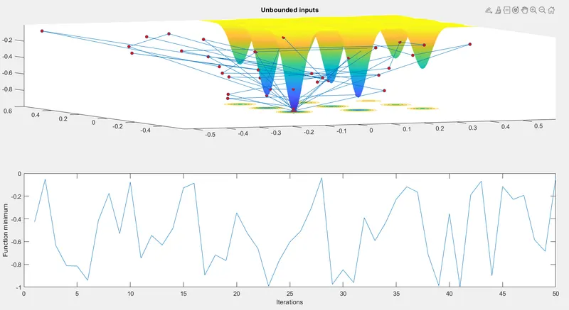
The output of study case1 shows the minimum and maximum values of stalagmite function that there is no bounds or constrains provided so the output values is different for each time we execute the program.

x = ga(fun,nvars) finds a local unconstrained minimum, fun,nvars is the dimension (number of design variables) of fun.

Study2 Result:

In the first case there was no bounds or constrains to the input parameters, to solve this issue study2 is used as the lower and upper values are bounded which is done by syntax as shown,

x = ga(fun,nvars,A,b,Aeq,beq)

which finds a local minimum x to fun, subject to the linear equalities Aeq*x = beq and A*x ≤ b.

Set A=[] and b=[] if no linear inequalities exist. ga evaluates the matrix product Aeq*x as if x is transposed (Aeq*x')

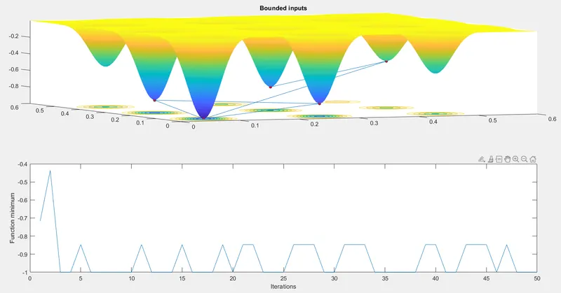
In the result file we can clearly see that the global maxima points has been shown in very few points when compared to the case study1.

Study3 Result:

The study case2 has few points of global maxima, hence in the study3 in addition to the bound initial population size is also given to get optimum maxima points. The default number of samplings has been initailly provided as 50, in study3 the population size is mentioned as 170 and the results as below

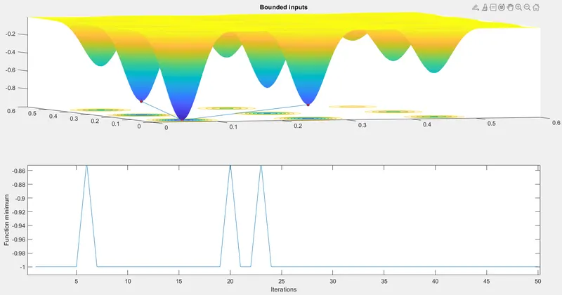
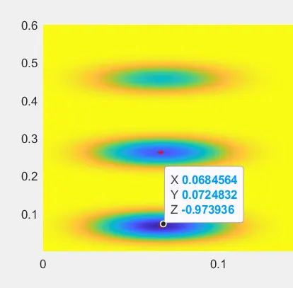
Result data for study3.

x = 0.068;

y = 0.072, this are the maxima values of stalagmite function.

Conclusion:

From the above procedure we can clearly understand the Genetic Algorithm, Optimization, Function of stalagmite expression and use of upper & lower bounds to constrain the values, plotting the maxima values. Hence, Genetic Algorithm uses randam values and it helps to get the best possible output. Stalagmite function always gives the minima values but th epurpose of maxima values has been taken.

Reference:

https://skill-lync.com/knowledgebase/genetic-algorithm-explained

https://in.mathworks.com/help/gads/ga.html#mw_4a8bfdb9-7c4c-4302-8f47-d260b7a43e26

https://in.mathworks.com/discovery/genetic-algorithm.html

https://www.tutorialspoint.com/genetic_algorithms/genetic_algorithms_introduction.htm