Project 1
AIM:
The task of this project is to compute the fuel economy numbers for the given vehicle (kmpl) on the urban cycle (UDDS) and highway cycle (HWFET). Also, to analyze and understand the vehicle operating
OBJECTIVE:
To develop the vehicle operating conditions. The model has some incomplete those are enigine and vehicle dynamics. Develop these two models and get the outputs from the simulink model. i.e Engine feul consumption, Distance travelled and the velocity of vehicle.In addition to that plot the outputs.
I need to test the vehicle Operation conditions for two different drive cycles. 1.UDDS, 2.HWFET
1. UDDS CYCLE :
Drive cycle is the vehicle velocity over a time.
UDDs stand for Urban dynamometer drive schedule.
It is testing the vechicle how it is driven in a city or urban driven conditions. Initially it starts with cold start and driven in stop and go. we all know that there is so many signals and so much of traffic in city's in that particular conditions this drive cycle is designed.
It is used for mostly for testing the light duty vehicles. from this drive cycle we can know the what is the fuel consumption, emission rate and vehicle thermal conditon in those driving conditions.The speed is set to 50 km/hr.
CODING PART:
Initial file of project
%%%%%%%%%%%%%%%%%%%%%%%%%%%%%%%%%%%%%%%%%%%%%%%%%%%%%%%%%%%%%%%%%%%%%
%% Skill-Lync -> Hybrid Drives Development
% Project 1 - Conventional Vehicle Model
% By - Ullekh Gambhira

% Description:

%% Initialization File
% Initialization file for loading the variables for the Conventional vehicle simulation model

%% Vehicle Parameters
M = 1500;       % Vehicle weight [kg]
Cr = 0.015;     % Rolling resistance coefficient
Rw = 0.35;      % Rolling radius [m]
Cd = 0.33;      % Drag coefficient
Af = 2;         % Frontal area [m2]
rhoa = 1.225;   % Air density [kg/m3]
Vwind = 0;      % Wind velocity [kmph]
g = 9.81;       % Gravitational acceleration [m/s2]
theta = 0;      % Slope [deg]
myu_road_tire = 1; % Coefficient of friction between tire - road interface

%% Powertrain Parameters
FDR = 3.73;                         % Final Drive Ratio / Diff Ratio
DiffEff = 0.99;                     % Differential efficiency (assumed independent of operating conditions)

NumGear = 4;                        % Number of gears in transmission
TransGear = [1:NumGear];            % Transmission Gears
TransRatio = [3.06, 1.62, 1, 0.7];  % Corresponding Transmission ratios
TransEff = 0.90;                    % Transmission efficiency (assumed independent of operating conditions)

TC_SR = [0, .5, .6, .7, .8, .87, .92, .94, .96, .97, 1];   % Torque Converter Speed Ratio (Matlab default) -> TurbSpd/PumpSpd
TC_TR = [2.232, 1.5462, 1.4058, 1.2746, 1.1528, 1.0732, 1.0192, 1, 1, 1, 1];   % Torque Converter Torque Ratio (Matlab default) -> TurbTrq/PumpTrq
TC_Cf = 1e-4 * [.72558, .66322, .63463, .59042, .51331, .4144, .29287, .22444, .12186, .04386, 0]; % Torque Converter Capacity Factor (Matlab default) -> PumpTrq/PumpSpd^2 [Nm/rpm^2]

load Vehicle_Data/Engine_data_1_9L_Saturn_95kW
load Vehicle_Data/Trans_Shift_map

%% Driver Parameters
Kp = 10;                    % P gain for driver PI model
Ki = 1;                     % I gain for driver PI model
Drive_Cycle_Select = 1;     % Drive cycle selection

% Drive cycle values in m/s

if Drive_Cycle_Select == 1
    load DriveCycles/UDDS;

elseif Drive_Cycle_Select == 2
    load DriveCycles/HWFET;

elseif Drive_Cycle_Select == 3
    load DriveCycles/FTP;

elseif Drive_Cycle_Select == 4
    load DriveCycles/US06;

elseif Drive_Cycle_Select == 5
    load DriveCycles/NEDC;

elseif Drive_Cycle_Select == 6
    load DriveCycles/WLTP;

end

time_end = cyc_time(end);
vel_end = cyc_vel(end);
Processing file
%%%%%%%%%%%%%%%%%%%%%%%%%%%%%%%%%%%%%%%%%%%%%%%%%%%%%%%%%%%%%%%%%%%%%
%% Skill-Lync -> Hybrid Drives Development
% Project 1 - Conventional Vehicle Model
% By - Ullekh Gambhira

% Description:
% The following file is to used with the Initialization file and Simulink
% results for post-processing of the data.
% The file is incomplete, has some examples of how the data is imported
% into a readable format, data analysis and plotting examples.
% Based on the project task, use commands in a similar format as given
% below, to analyse the data and generate required plots.
% You can change variable names if desired

%% Post-Processing File
%  File for post-processing the Conventional vehicle simulation model data

%% Renaming variables
Time = out.tout;
Acc_Pdl = out.Acc_Pdl;          % Accelerator pedal [%]
Brk_Pdl = out.Brk_Pdl;          % Brake pedal [%]
Gear_Cmd = out.Gear_Cmd;        % Transmission gear
Trans_In_Spd = out.Trans_In_Spd*30/pi;  % Transmission input speed [rpm]
Trans_Out_Spd = out.Trans_Out_Spd*30/pi;% Transmission output speed [rpm]
Eng_Trq = out.Eng_Trq;          % Engine brake torque [Nm]
Eng_Spd = out.Eng_Spd*30/pi;    % Engine speed [rpm]
Eng_Fuel_Consump = out.Eng_Fuel_Consumption;    % Engine fuel consumption [g]
Veh_Dist = out.Veh_Dist/1000;   % Distance traveled by vehicle [km]
Veh_Spd = out.Veh_Spd*18/5;     % Vehicle speed [kmph]


%% Data Analysis
Eng_Pwr = Eng_Spd*pi/30*Eng_Trq/1000;   % Engine brake power [kW]
rho_petrol = 0.7197;                    % Density of petrol [kg/L]
% kmpl = Veh_Dist(end)/(Eng_Fuel_Consump(end)/1000/rho_petrol);    % Fuel economy [kmpl]


%% Plotting vehicle characteristics time trace
figure()
subplot(3,1,1)
hold on
grid on
plot(Time, Acc_Pdl, 'linewidth', 1, 'Color', 'black');
plot(Time, Brk_Pdl, 'linewidth', 1, 'Color', 'red');
ylabel('Pedal [%]')
xlim([0, Time(end)]);
legend('Accel','Brake');
subplot(3,1,2)
hold on
grid on
plot(Time, Trans_In_Spd, 'linewidth', 1, 'Color', 'black');
plot(Time, Trans_Out_Spd, 'linewidth', 1, 'Color', 'red');
ylabel('Speed [rpm]')
xlim([0, Time(end)]);
ylim([0, 6000]);
legend('Trans Input','Trans Output');
subplot(3,1,3)
hold on
grid on
plot(Time, Gear_Cmd, 'linewidth', 1, 'Color', 'black');
xlim([0, Time(end)]);
xlabel('Time [s]');
ylabel('Gear');

%% Plotting engine operating points on engine fuel map
figure('Name','Engine Operating Points');
hold on
grid on
title('Engine Operating Points','fontsize',12);
p1=plot(Eng_map_spd*30/pi,Eng_max_trq,'linewidth',2,'color','r');
p2=line([Eng_map_spd(end)*30/pi Eng_map_spd(end)*30/pi],[0 Eng_max_trq(end)]);
set(p2,'linewidth',1,'linestyle','--','color','k');
p3=line([Eng_map_spd(1)*30/pi Eng_map_spd(1)*30/pi],[0 Eng_max_trq(1)]);
set(p3,'linewidth',1,'linestyle','--','color','k');
[c,h] = contour(Eng_map_spd'*30/pi,Eng_map_trq,Eng_fuel_map');
clabel(c,h);
xlabel('Engine Speed [rpm]');
ylabel('Engine Torque [Nm]');
title('Engine Fuel Consumption Map [g/s]');
p4 = plot(Eng_Spd,Eng_Trq,'.','color','k');
legend([p1 p4],{'Max Curve','Operating Points'});
axis([Eng_map_spd(1)*30/pi Eng_map_spd(end)*30/pi 0 Eng_map_trq(end)]);
RESULTS :
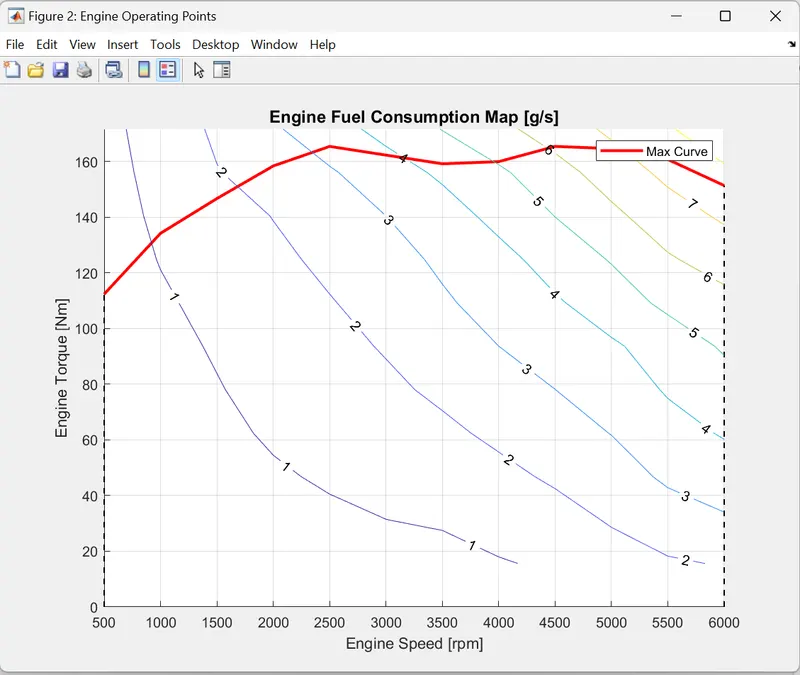
Plotting engine torque, engine power, fuel rate and fuel consumption here the max curve shows the fuel consumption for the particular speed and torque values. the fuel consumption is max when the speed of vehicle increases and the fuel flow rate also increases .
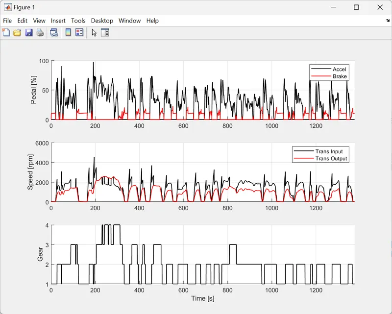
In subplotting
Plotting of accelerator and brake pedal, gear command, vehicle desired and actual speed, vehicle distance. The shorter distance the accelaration gets incressed and the vehicle is to be pull overed suddenly usually the brakes are applied to controll the vehicle then vehicle is come zero speed and again started from zero reach some distance and come to zero. There is an ideilling losses in this cycle.
Plotting the time trace for engine, transmission input, transmission output and wheel speed. here in this case input power is more than the output. actually what happens is the input power is trying to match the output power with in a time the vehicle gets pull overed. beacuse of a start-go stop.
2. HWFET CYCLE :
HIGHWAY FUEL ECONOMY TESTING Schedule
This cycle is US based high way cycle it combination of highway driving and Rural. The cycle is started with the warmed up engine cycle is completely free of traffic. This vehicle operates with the sped of 74 km/hr the time interval is also set for the cycle.
CODING PART :
Initial ile for project HWFET cycle
%%%%%%%%%%%%%%%%%%%%%%%%%%%%%%%%%%%%%%%%%%%%%%%%%%%%%%%%%%%%%%%%%%%%%
%% Skill-Lync -> Hybrid Drives Development
% Project 1 - Conventional Vehicle Model
% By - Ullekh Gambhira

% Description:

%% Initialization File
% Initialization file for loading the variables for the Conventional vehicle simulation model

%% Vehicle Parameters
M = 1500;       % Vehicle weight [kg]
Cr = 0.015;     % Rolling resistance coefficient
Rw = 0.35;      % Rolling radius [m]
Cd = 0.33;      % Drag coefficient
Af = 2;         % Frontal area [m2]
rhoa = 1.225;   % Air density [kg/m3]
Vwind = 0;      % Wind velocity [kmph]
g = 9.81;       % Gravitational acceleration [m/s2]
theta = 0;      % Slope [deg]
myu_road_tire = 1; % Coefficient of friction between tire - road interface

%% Powertrain Parameters
FDR = 3.73;                         % Final Drive Ratio / Diff Ratio
DiffEff = 0.99;                     % Differential efficiency (assumed independent of operating conditions)

NumGear = 4;                        % Number of gears in transmission
TransGear = [1:NumGear];            % Transmission Gears
TransRatio = [3.06, 1.62, 1, 0.7];  % Corresponding Transmission ratios
TransEff = 0.90;                    % Transmission efficiency (assumed independent of operating conditions)

TC_SR = [0, .5, .6, .7, .8, .87, .92, .94, .96, .97, 1];   % Torque Converter Speed Ratio (Matlab default) -> TurbSpd/PumpSpd
TC_TR = [2.232, 1.5462, 1.4058, 1.2746, 1.1528, 1.0732, 1.0192, 1, 1, 1, 1];   % Torque Converter Torque Ratio (Matlab default) -> TurbTrq/PumpTrq
TC_Cf = 1e-4 * [.72558, .66322, .63463, .59042, .51331, .4144, .29287, .22444, .12186, .04386, 0]; % Torque Converter Capacity Factor (Matlab default) -> PumpTrq/PumpSpd^2 [Nm/rpm^2]

load Vehicle_Data/Engine_data_1_9L_Saturn_95kW
load Vehicle_Data/Trans_Shift_map

%% Driver Parameters
Kp = 10;                    % P gain for driver PI model
Ki = 1;                     % I gain for driver PI model
Drive_Cycle_Select = 2;     % Drive cycle selection

% Drive cycle values in m/s

if Drive_Cycle_Select == 1
    load DriveCycles/UDDS;

elseif Drive_Cycle_Select == 2
    load DriveCycles/HWFET;

elseif Drive_Cycle_Select == 3
    load DriveCycles/FTP;

elseif Drive_Cycle_Select == 4
    load DriveCycles/US06;

elseif Drive_Cycle_Select == 5
    load DriveCycles/NEDC;

elseif Drive_Cycle_Select == 6
    load DriveCycles/WLTP;

end

time_end = cyc_time(end);
vel_end = cyc_vel(end);
Plotting file
%%%%%%%%%%%%%%%%%%%%%%%%%%%%%%%%%%%%%%%%%%%%%%%%%%%%%%%%%%%%%%%%%%%%%
%% Skill-Lync -> Hybrid Drives Development
% Project 1 - Conventional Vehicle Model
% By - Ullekh Gambhira

% Description:
% The following file is to used with the Initialization file and Simulink
% results for post-processing of the data.
% The file is incomplete, has some examples of how the data is imported
% into a readable format, data analysis and plotting examples.
% Based on the project task, use commands in a similar format as given
% below, to analyse the data and generate required plots.
% You can change variable names if desired

%% Post-Processing File
%  File for post-processing the Conventional vehicle simulation model data

%% Renaming variables
Time = out.tout;
Acc_Pdl = out.Acc_Pdl;          % Accelerator pedal [%]
Brk_Pdl = out.Brk_Pdl;          % Brake pedal [%]
Gear_Cmd = out.Gear_Cmd;        % Transmission gear
Trans_In_Spd = out.Trans_In_Spd*30/pi;  % Transmission input speed [rpm]
Trans_Out_Spd = out.Trans_Out_Spd*30/pi;% Transmission output speed [rpm]
Eng_Trq = out.Eng_Trq;          % Engine brake torque [Nm]
Eng_Spd = out.Eng_Spd*30/pi;    % Engine speed [rpm]
Eng_Fuel_Consump = out.Eng_Fuel_Consumption;    % Engine fuel consumption [g]
Veh_Dist = out.Veh_Dist/1000;   % Distance traveled by vehicle [km]
Veh_Spd = out.Veh_Spd*18/5;     % Vehicle speed [kmph]


%% Data Analysis
Eng_Pwr = Eng_Spd*pi/30*Eng_Trq/1000;   % Engine brake power [kW]
rho_petrol = 0.7197;                    % Density of petrol [kg/L]
% kmpl = Veh_Dist(end)/(Eng_Fuel_Consump(end)/1000/rho_petrol);    % Fuel economy [kmpl]


%% Plotting vehicle characteristics time trace
figure()
subplot(3,1,1)
hold on
grid on
plot(Time, Acc_Pdl, 'linewidth', 1, 'Color', 'black');
plot(Time, Brk_Pdl, 'linewidth', 1, 'Color', 'red');
ylabel('Pedal [%]')
xlim([0, Time(end)]);
legend('Accel','Brake');
subplot(3,1,2)
hold on
grid on
plot(Time, Trans_In_Spd, 'linewidth', 1, 'Color', 'black');
plot(Time, Trans_Out_Spd, 'linewidth', 1, 'Color', 'red');
ylabel('Speed [rpm]')
xlim([0, Time(end)]);
ylim([0, 6000]);
legend('Trans Input','Trans Output');
subplot(3,1,3)
hold on
grid on
plot(Time, Gear_Cmd, 'linewidth', 1, 'Color', 'black');
xlim([0, Time(end)]);
xlabel('Time [s]');
ylabel('Gear');

%% Plotting engine operating points on engine fuel map
figure('Name','Engine Operating Points');
hold on
grid on
title('Engine Operating Points','fontsize',12);
p1=plot(Eng_map_spd*30/pi,Eng_max_trq,'linewidth',2,'color','r');
p2=line([Eng_map_spd(end)*30/pi Eng_map_spd(end)*30/pi],[0 Eng_max_trq(end)]);
set(p2,'linewidth',1,'linestyle','--','color','k');
p3=line([Eng_map_spd(1)*30/pi Eng_map_spd(1)*30/pi],[0 Eng_max_trq(1)]);
set(p3,'linewidth',1,'linestyle','--','color','k');
[c,h] = contour(Eng_map_spd'*30/pi,Eng_map_trq,Eng_fuel_map');
clabel(c,h);
xlabel('Engine Speed [rpm]');
ylabel('Engine Torque [Nm]');
title('Engine Fuel Consumption Map [g/s]');
p4 = plot(Eng_Spd,Eng_Trq,'.','color','k');
legend([p1 p4],{'Max Curve','Operating Points'});
axis([Eng_map_spd(1)*30/pi Eng_map_spd(end)*30/pi 0 Eng_map_trq(end)]);
RESULTS :
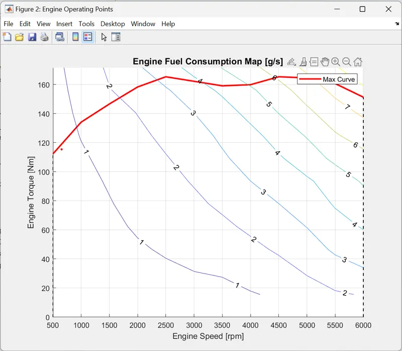
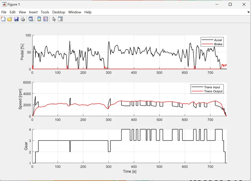
The plots clearly showing that the plots accelaration and bake pedal with the time. In the plotting accelaration is started with heat start and it get down at some stages and raise for different time intervals and the brake is applied in small stages untill the cycle is running through out the time interval.
The plotting input speed is reched to the output speed and there some loss in intial time and after that the vehicle get reached the input what get generated this is a big cycle and the vehicle is operated in those conditions.
CONSLUTION :
Hence the Engine and the vehicle dynamics are modeled in simulink.
The ouput from the model are get saved in workspace
Plotting for different parameters are also done.
The both cycles are having two different cycles may varry the fuel consumption and emission rate.