Project 1
Title:-
Deals with the development of a forward energy-based fuel consumption model of a conventional vehicle.
Aim:-
1] Build Simulink model using blocks and complete the vehicle model.
2] Writting scripts in MATLAB to load all the variables required for running the Simulink model.
3] Tabulate the fuel economy numbers (kmpl) for UDDS and HWFET cycle.
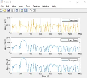
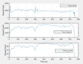
4] Plot the time trace for engine, transmission input, transmission output and wheel speed on one plot.
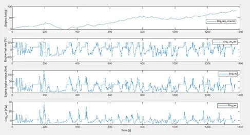
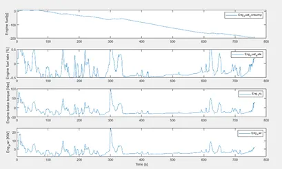
5] Plot engine torque, engine power, fuel rate and fuel consumption using subplots.
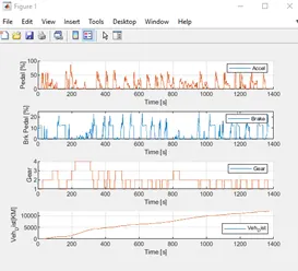
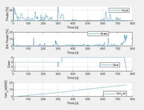
6] Plot accelerator and brake pedal, gear command, vehicle desired and actual speed, vehicle distance using subplots.
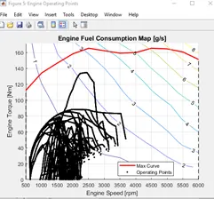
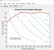
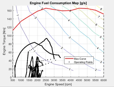
7] Plot the engine operating points on the engine fuel map.
8] Generate the plots for both drive cycles.
9] Study of Conventional vehicle simulink model and creates graphs.
Conventional Vehicle Forward Model:-
It also known as dynamic simulation. Dynamic models are used for detailed simulations. In this model force/torque/power is the input and the vehicle state variable velocity and acceleration are outputs. The models and simulatios are more realistic due to phisical casualty hence appropriate for control development. There is feedback loop to meet the desired vehicle state. It is mainly used to simulate a vehicle on a driving cycle to analyse the dynamic behaviour of the system helps significantly in control development.
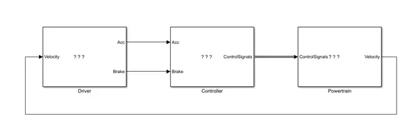
1.Drive Model-
Drive model is the driver inputs to the controller, brake & acceleration given as a inputs to the controller. This Block is created with help of drive cycle lookup table & PID controller for correcting error signal of the feedback velocity signal, generated the Acc_pdl & Brk_pdl as output through the saturation block. These signals given as input to the controller block.
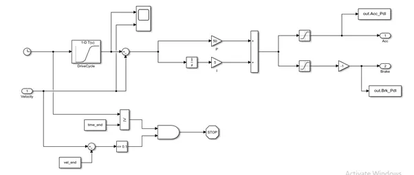
2.Controller-
Controller block having sub blocks Engine ,Transmission & Brake, vehicle velocity ,acceleration & brake signals given as inputs to the these blocks, controller block generate the output as Engine Torque, Gear command & required brake torque.
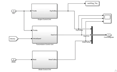
1.Engine Control-
Engine control block takes the engine speed as input & gives the engine required torque as output with help of lookup blocks.
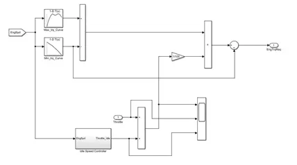
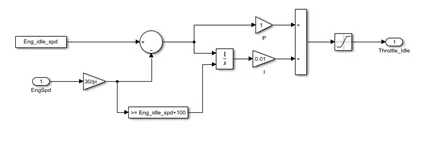
Idle Engine Speed controller-
2.Transmission Control-
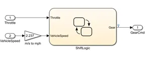
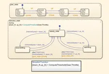
Transmission control block is created using shift logic block ,vehicle speed & Throttle given as input & Gear command taken as output of the of the transmission control block, shift logic designed based on the vehicle speed & it will shift the gear 1-4 based operating region of the input speed. Simulink function block used for selection state shift block.
3.Brake Control-
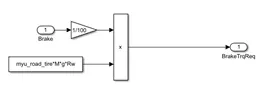
Based on the appied brake & rolling resistance calculated the Brake torque.
3.Power Train-
The powertrain encompasses every component that converts the engine's power into movement. This includes the engine, transmission, the driveshaft, differentials, axles; basically anything from the engine through to the rotating wheel
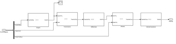
1)Engine-
In this model we used map based model to model the fuel consumption of engine. It is based on maximum Torque and minimum torque from the controller. and then it saturated torque and give output then saturated torque and speed map give fuel consumption takes the speed and torque then the output goes into saturated then its integrated.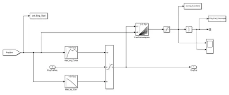
2)Transmission—
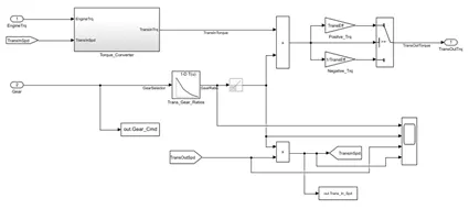
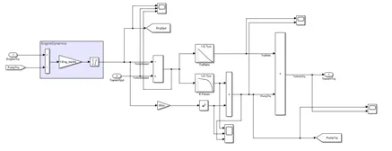
In these model we take engine torque, gear selector from controller signal for transmission of gear ratio. The ratio is multiply by transmission input torque and then the transmission efficiency positive torque and negative torque gives transmission input speed. In this case torque converter connects the engine to transmission it is part of transmission.
Torque converter-
3)Differential—
In this taking input is the transmission output then its going to the differential ratio multiplied the output and input torque then meet axle torque. The axle torque is a lower than the transmission torque and differential ratio.
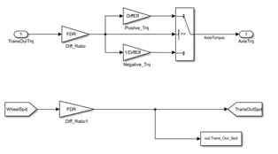
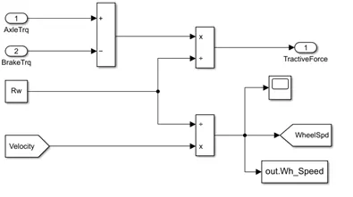
4)Wheels—
In this model we take the axle torque from differentail & brake torque from controller. it is substracted and multiplied rolling radius and velocity then we meet the tractive force from axle and brake torque. Wheel block give the wheel speed signal as output.
5) Vehicle Dynamics—
Vehicle Dynamics block designed based on the below dynamic equation (tractive force and road load) this block generates the vehicle velocity, vehicle distance as output from the block, this output vehicle velocity given to the drive block as a feedback signal

The dynamic equation for designing the Vehicle dynamic block is
where,
p = air density [kg/m^3]
A = Frontal area [m^2]
Cd = drag Coefficiend
Vveh = velocity of vehicle [m/s^2]
Vwind = velocity of wind [m/s^2]
Cr = rolling resistance coefficient
M = mass in [Kg]
g = gravity.
MATLAB scripts:-
Used to load all the variables required for running the Simulink model and for post-processing. The drive cycle selection is also done here. Before running the Simulink vehicle model, run this initialization script.
%%%%%%%%%%%%%%%%%%%%%%%%%%%%%%%%%%%%%%%%%%%%%%%%%%%%%%%%%%%%%%%%%%%%%
%% Skill-Lync -> Hybrid Drives Development
% Project 1 - Conventional Vehicle Model
% By - Guruprasad Joshi
% Description:
%% Initialization File
% Initialization file for loading the variables for the Conventional vehicle simulation model
%% Vehicle Parameters
M = 1500; % Vehicle weight [kg]
Cr = 0.015; % Rolling resistance coefficient
Rw = 0.35; % Rolling radius [m]
Cd = 0.33; % Drag coefficient
Af = 2; % Frontal area [m2]
rhoa = 1.225; % Air density [kg/m3]
Vwind = 0; % Wind velocity [kmph]
g = 9.81; % Gravitational acceleration [m/s2]
theta = 0; % Slope [deg]
myu_road_tire = 1; % Coefficient of friction between tire - road interface
%% Powertrain Parameters
FDR = 3.73; % Final Drive Ratio / Diff Ratio
DiffEff = 0.99; % Differential efficiency (assumed independent of operating conditions)
NumGear = 4; % Number of gears in transmission
TransGear = [1:NumGear]; % Transmission Gears
TransRatio = [3.06, 1.62, 1, 0.7]; % Corresponding Transmission ratios
TransEff = 0.90; % Transmission efficiency (assumed independent of operating conditions)
TC_SR = [0, .5, .6, .7, .8, .87, .92, .94, .96, .97, 1]; % Torque Converter Speed Ratio (Matlab default) -> TurbSpd/PumpSpd
TC_TR = [2.232, 1.5462, 1.4058, 1.2746, 1.1528, 1.0732, 1.0192, 1, 1, 1, 1]; % Torque Converter Torque Ratio (Matlab default) -> TurbTrq/PumpTrq
TC_Cf = 1e-4 * [.72558, .66322, .63463, .59042, .51331, .4144, .29287, .22444, .12186, .04386, 0]; % Torque Converter Capacity Factor (Matlab default) -> PumpTrq/PumpSpd^2 [Nm/rpm^2]
load Vehicle_Data/Engine_data_1_9L_Saturn_95kW
load Vehicle_Data/Trans_Shift_map
%% Driver Parameters
Kp = 10; % P gain for driver PI model
Ki = 1; % I gain for driver PI model
Drive_Cycle_Select = 2; % Drive cycle selection
% Drive cycle values in m/s
if Drive_Cycle_Select == 1
load DriveCycles/UDDS;
elseif Drive_Cycle_Select == 2
load DriveCycles/HWFET;
elseif Drive_Cycle_Select == 3
load DriveCycles/FTP;
elseif Drive_Cycle_Select == 4
load DriveCycles/US06;
elseif Drive_Cycle_Select == 5
load DriveCycles/NEDC;
elseif Drive_Cycle_Select == 6
load DriveCycles/WLTP;
end
time_end = cyc_time(end);
vel_end = cyc_vel(end);
MATLAB scripts for plots:-
%%%%%%%%%%%%%%%%%%%%%%%%%%%%%%%%%%%%%%%%%%%%%%%%%%%%%%%%%%%%%%%%%%%%%
%% Skill-Lync -> Hybrid Drives Development
% Project 1 - Conventional Vehicle Model
% By - Guruprasad Joshi
%% Post-Processing File
% File for post-processing the Conventional vehicle simulation model data
%% Renaming variables
Time=out.tout;
Acc_Pdl=out.Acc_Pdl; % Accelerator pedal [%]
Brk_Pdl=out.Brk_Pdl; % Brake pedal [%]
Gear_Cmd=out.Gear_Cmd; % Transmission gear
Trans_In_Spd=out.Trans_In_Spd*30/pi; % Transmission input speed [rpm]
Trans_Out_Spd=out.Trans_Out_Spd*30/pi;% Transmission output speed [rpm]
Eng_Trq=out.Eng_Trq; % Engine brake torque [Nm]
Eng_Spd=out.Eng_Spd*30/pi; % Engine speed [rpm]
Eng_Fuel_Consump=out.Eng_Fuel_Consumption; % Engine fuel consumption [g]
Veh_Dist=out.Veh_Dist/1000; % Distance traveled by vehicle [km]
Veh_Spd=out.Veh_Spd*18/5; % Vehicle speed [kmph]
Wheel_Speed=out.Wh_Speed; % Wheel speed [kmph]
Eng_Fuel_Rate=out.Eng_Fuel_Rate % Engine fuel rate [%]
%% Data Analysis
Eng_Pwr=Eng_Spd*(pi/30).*(Eng_Trq/1000); % Engine brake power [kW]
rho_petrol=0.7197; % Density of petrol [kg/L]
%kmpl=Veh_Dist/(Eng_Fuel_Consump/1000/rho_petrol); % Fuel economy [kmpl]
%% Plotting vehicle characteristics time trace
figure(1)
subplot(411)
hold on
grid on
plot(Time,Acc_Pdl);
ylabel('Pedal [%]');
xlabel('Time [s]');
legend('Accel');
subplot(412)
plot(Time,Brk_Pdl);
ylabel('Brk Pedal [%]')
xlabel('Time [s]');
legend('Brake');
subplot(413)
hold on
grid on
plot(Time,Gear_Cmd);
xlabel('Time [s]');
ylabel('Gear');
legend('Gear');
subplot(414)
hold on
grid on
plot(Time,Veh_Dist);
xlabel('Time [s]');
ylabel('Veh_Dist[KM]');
legend('Veh_Dist');
figure(2)
subplot(311)
hold on
grid on
plot(Time,Trans_In_Spd);
ylabel('Speed [rpm]')
legend('Trans Input');
subplot(312)
plot(Time,Trans_Out_Spd);
ylabel('Speed [rpm]')
legend('Trans Output');
subplot(313)
plot(Time,Wheel_Speed);
ylabel('Speed [rpm]')
xlabel('Time [s]');
legend('Wheel_Speed');
figure(3)
subplot(411)
plot(Time,Eng_Fuel_Consump);
ylabel('Engine fuel[g]')
legend('Eng_Fuel_Consump')
subplot(412)
plot(Time,Eng_Fuel_Rate);
ylabel('Engine fuel rate [%]')
legend('Eng_Fuel_Rate');
subplot(413)
plot(Time,Eng_Trq)
ylabel('Engine brake torque [Nm]')
legend('Eng_Trq');
subplot(414)
plot(Time,Eng_Pwr);
ylabel('Eng_Pwr [KW]')
xlabel('Time [s]');
legend('Eng_Pwr');
%% Plotting engine operating points on engine fuel map
figure('Name','Engine Operating Points');
hold on
grid on
title('Engine Operating Points','fontsize',12);
p1=plot(Eng_map_spd*30/pi,Eng_max_trq,'linewidth',2,'color','r');
p2=line([Eng_map_spd(end)*30/pi Eng_map_spd(end)*30/pi],[0 Eng_max_trq(end)]);
set(p2,'linewidth',1,'linestyle','--','color','k');
p3=line([Eng_map_spd(1)*30/pi Eng_map_spd(1)*30/pi],[0 Eng_max_trq(1)]);
set(p3,'linewidth',1,'linestyle','--','color','k');
[c,h] = contour(Eng_map_spd'*30/pi,Eng_map_trq,Eng_fuel_map');
clabel(c,h);
xlabel('Engine Speed [rpm]');
ylabel('Engine Torque [Nm]');
title('Engine Fuel Consumption Map [g/s]');
p4 = plot(Eng_Spd,Eng_Trq,'.','color','k');
legend([p1 p4],{'Max Curve','Operating Points'});
axis([Eng_map_spd(1)*30/pi Eng_map_spd(end)*30/pi 0 Eng_map_trq(end)]);
Graphs for the drive cycle UDDS
1] Plot accelerator and brake pedal, gear command, and actual speed, vehicle distance using subplots.
2] Plot the time trace for engine, transmission input, transmission output and wheel speed on one plot
3] Plot engine torque, engine power, fuel rate and fuel consumption using subplots.
4] Plot the engine operating points on the engine fuel map.
Graphs for the drive cycle HWFEET
1] Plot accelerator and brake pedal, gear command, and actual speed, vehicle distance using subplots.
2] Plot the time trace for engine, transmission input, transmission output and wheel speed on one plot
3] Plot engine torque, engine power, fuel rate and fuel consumption using subplots.
4] Plot the engine operating points on the engine fuel map.
Conclusion:
Completed the conventional vehicle modelling design by creating the Engine & vehicle dynamic blocks, also added the work space & scope blocks to analyse the results. With help of MATLAB script plotted the various parameters of the vehicle model such as engine torque, engine power, fuel rate and fuel consumption, transmission input, transmission output and wheel speed, accelerator and brake pedal, gear command, and actual speed, vehicle distance & engine operating points on the engine fuel map for the drive cycle data of UDDS & HWFET.
Fuel consumption is more in UDDS drive cycle compare to HWFET drive cycle this data we have analysed based on the graphs.