Problem Set-1 c Week 11Challenge : Transient Handling
The following table contains information about two vehicles
FWD passenger car:
Code:
clear all
close all
clc

l = 2.538984 ; %Wheelbase (m)
a = 0.890016; %cg to front axle (m)
b = l-a; %cg to rear axle (m)
m = 907.18474; %Mass (kg)
jz = 1128 ; %moment of inertia (kg-m^2)
cf = 61171.9437; %front cornering stiffness (N/rad)
cr = 50976.6191; %rear cornering stiffness (N/rad)
u = 100/3.6;
A=[-(cf+cr)/(m*u),(((b*cr)-(a*cf))/(m*u))-u;((b*cr)-(a*cf))/(jz*u),-((((a^2)*cf)+((b^2)*cr))/(jz*u))];
B=[cf/m;(a*cf)/jz];

%lateral speed
c1=[1,0];
d1=0;

% yaw rate
c2=[0,1];
d2=0;

%lateral acceleration
c3=A(1,:)+u*[0,1];
d3=B(1);

t=(0:0.01:2);
steering=(pi/180)*5*sin(2*pi*7*t);

C=[c1;c2;c3];
D=[d1;d2;d3];

%space-state
sys=ss(A,B,C,D);

Y=lsim(sys,steering,t);

sys.Inputname={'steering'};
sys.Outputname={'lateral speed','yaw rate','lateral acceleration'};

[mag,phase,omega] = bode(sys({'yaw rate'},{'steering'}));

for i=1:length(mag)
magnitude(i)=mag(1,1,i);
end

figure(1)
loglog(omega/(2*pi),magnitude,'linewidth',2)
title('yaw gain frequency response')
xlabel('Frequency (Hz)')
ylabel('Gain')
grid on

figure(2)
subplot(2,2,1)
plot(t,steering,'linewidth',2)
title('Steering')
xlabel('Time (s)')
ylabel('Steering angle (rad)')
grid on

subplot(2,2,2)
plot(t,Y(:,1),'linewidth',2)
title('Lateral speed')
xlabel('Time (s)')
ylabel('Lateral speed (m/s)')
grid on


subplot(2,2,3)
plot(t,Y(:,2),'linewidth',2)
title('Yaw rate')
xlabel('Time (s)')
ylabel('Yaw rate (rad/sec)')
grid on


subplot(2,2,4)
plot(t,Y(:,3),'linewidth',2)
title('Lateral accelaration')
xlabel('Time (s)')
ylabel('Lateral accelration (m/s^2)')
grid on

figure(3)
step(sys)
grid on


S=stepinfo(sys);

[wn, theta]=damp(sys);

Cf = -61171.9437; %front cornering stiffness (N/rad)
Cr = -50976.6191; %rear cornering stiffness (N/rad)

YB=Cf+Cr;
YR=(a*Cf-b*Cr)/u;
YS=-Cf;
NB=a*Cf-b*Cr;
NR=(((a^2)*Cf)+((b^2)*Cr))/u;
NS=-a*Cf;

Wn=sqrt(((YB*NR)+(NB*m*u)-(YR*NB))/(m*u*jz));
Theta=abs(-((NR/jz)+(YB/(m*u)))*(1/(2*Wn)));
Wd=Wn*sqrt(1-(Theta)^2);
tr=((m*u*NS)/((YS*NB)-(YB*NS)));
Plot:
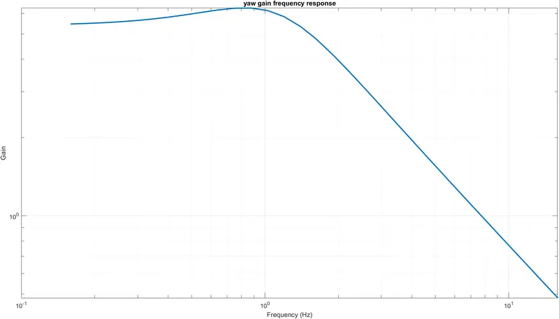
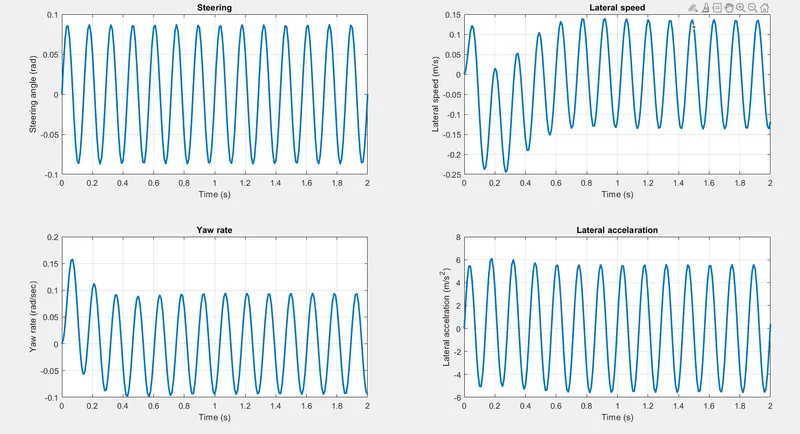
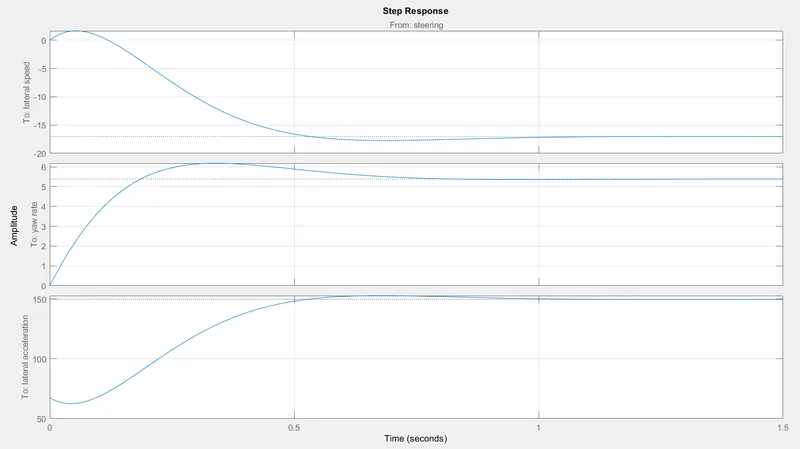
Correlation at 7Hz:
Gain (from yaw rate and steering rate) = 0.0935/0.0855 = 1.093
From frequency response it can be see that gain is approx. 1.1
Steady state yaw gain refers to the system's gain when t approaches infinity or at extremely low frequency; for example, in the step response, it achieves a steady state output value of 5.4 for a unity step input, therefore the steady state gain is 5.4.
Rise time correlation:
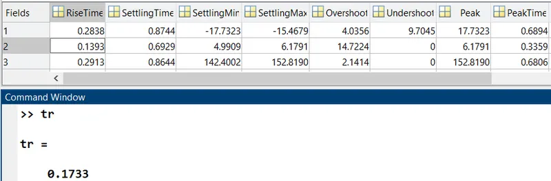
There is a minor difference between the analytical calculation of rise time and the automated calculation using the step info function in MATLAB, but it is acceptable.
Results:
YB=-1.125*10^5
YR=6.1172*10^4
YS=6.1172*10^4
NB=2.9615*10^4
NR=-6.7344*10^3
NS=5.4444*10^4
Wn=7.1912 rad/s
Theta=0.72245
Wd=4.9564 rad/s
tr=0.1733 s
F1 car
Code:
clear all
close all
clc

l = 2.901696 ; % Wheelbase (m)
a = 1.740408; % cg to front axle (m)
b = l-a; % cg to rear axle (m)
m = 779.725284; % Mass (kg)
jz = 865 ; % moment of inertia (kg-m^2)
cf = 276803.935; % front cornering stiffness (N/rad)
cr = 429733.794; % rear cornering stiffness (N/rad)
u = 100/3.6;

A=[-(cf+cr)/(m*u),(((b*cr)-(a*cf))/(m*u))-u;((b*cr)-(a*cf))/(jz*u),-((((a^2)*cf)+((b^2)*cr))/(jz*u))];
B=[cf/m;(a*cf)/jz];

%lateral speed
c1=[1,0];
d1=0;

% yaw rate
c2=[0,1];
d2=0;

%lateral acceleration
c3=A(1,:)+u*[0,1];
d3=B(1);

t=(0:0.01:2);
steering=(pi/180)*5*sin(2*pi*7*t);

C=[c1;c2;c3];
D=[d1;d2;d3];

%space-state
sys=ss(A,B,C,D);

Y=lsim(sys,steering,t);

sys.Inputname={'steering'};
sys.Outputname={'lateral speed','yaw rate','lateral acceleration'};

[mag,phase,omega] = bode(sys({'yaw rate'},{'steering'}));

for i=1:length(mag)
magnitude(i)=mag(1,1,i);
end

figure(1)
loglog(omega/(2*pi),magnitude,'linewidth',2)
title('yaw gain frequency response')
xlabel('Frequency (Hz)')
ylabel('Gain')
grid on

figure(2)
subplot(2,2,1)
plot(t,steering,'linewidth',2)
title('Steering')
xlabel('Time (s)')
ylabel('Steering angle (rad)')
grid on

subplot(2,2,2)
plot(t,Y(:,1),'linewidth',2)
title('Lateral speed')
xlabel('Time (s)')
ylabel('Lateral speed (m/s)')
grid on


subplot(2,2,3)
plot(t,Y(:,2),'linewidth',2)
title('Yaw rate')
xlabel('Time (s)')
ylabel('Yaw rate (rad/sec)')
grid on


subplot(2,2,4)
plot(t,Y(:,3),'linewidth',2)
title('Lateral accelaration')
xlabel('Time (s)')
ylabel('Lateral accelration (m/s^2)')
grid on

figure(3)
step(sys)
grid on


S=stepinfo(sys);

[wn, theta]=damp(sys);

Cf = -61171.9437; %front cornering stiffness (N/rad)
Cr = -50976.6191; %rear cornering stiffness (N/rad)

YB=Cf+Cr;
YR=(a*Cf-b*Cr)/u;
YS=-Cf;
NB=a*Cf-b*Cr;
NR=(((a^2)*Cf)+((b^2)*Cr))/u;
NS=-a*Cf;

Wn=sqrt(((YB*NR)+(NB*m*u)-(YR*NB))/(m*u*jz));
Theta=abs(-((NR/jz)+(YB/(m*u)))*(1/(2*Wn)));
Wd=Wn*sqrt(1-(Theta)^2);
tr=((m*u*NS)/((YS*NB)-(YB*NS)));
Output:
Correlation at 7 Hz:
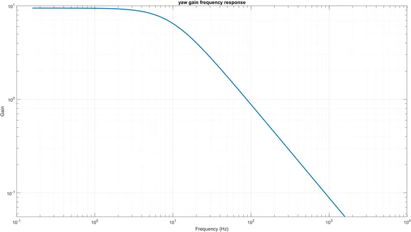
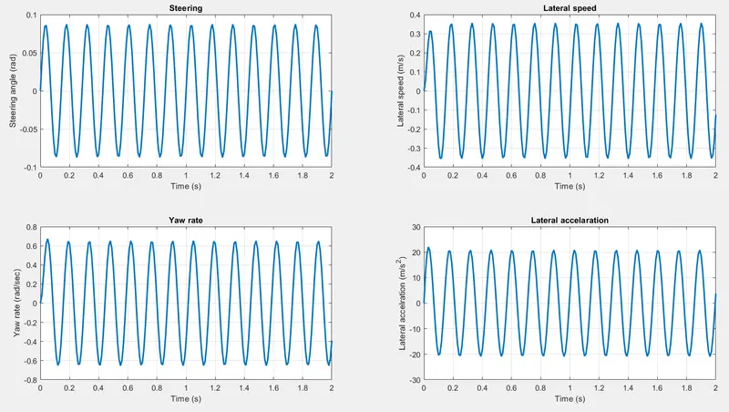
Gain (from yaw rate and steering rate) = 1.03/0.0855 = 12.04
From frequency response it can be see that gain is approx. 12.05
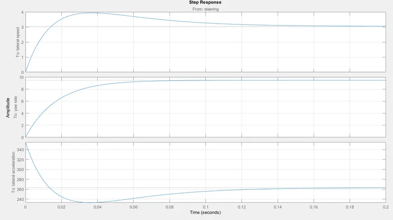
The steady state gain of 30 is found in the time plot as well as the frequency plot
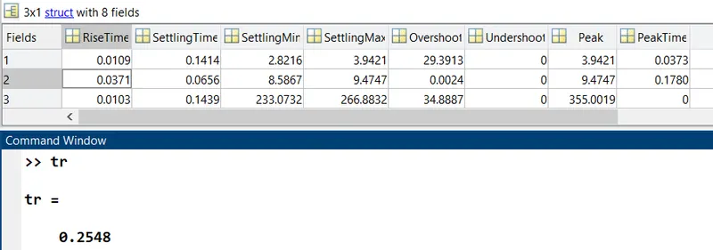
There is a minor difference between the analytical calculation of rise time and the automated calculation using the step info function in MATLAB, but it is acceptable.
Results:
YB=-7.0654*10^5
YR=177.87
YS=2.7680*10^5
NB=1.7293*10^4
NR=-1.4585*10^4
NS=4.8175*10^5
Wn=13.3077 rad/s
Theta=0.9837
Wd=2.3934 rad/s
tr=0.1058 s