Port Fuel Injection Engine Simulation
THEORY: Historically, the most widely produced internal combustion engines were of the Port Fuel Injected (PFI) design, where the fuel is sprayed into the intake ports to mix with incoming air. In fact, many new vehicles are still manufactured with this engine design. The fuel injectors in PFI configurations are typically mounted in the intake manifold and the air/fuel mixture is pulled into the cylinder head as the intake valve opens. Port fuel-injection systems long ago replaced carburettors in cars because of their efficiency and lower maintenance requirements. But now, automakers are moving towards the even more efficient direct injection. With port fuel injection, gasoline is sprayed into the intake manifold, where it mixes with air, and then is sucked down into the cylinders. Direct injection places an injector on each cylinder, spraying gasoline into the cylinder itself. Direct injection leads to more efficient engines, as the gasoline-air mixture burns more completely. The individual injectors also ensure that each cylinder gets the same amount of fuel, and the spray can be more precisely timed.
Spray modeling
Spray models are very important in engine CFD simulations because they influence the subsequent mixing, ignition, combustion and emission predictions. Spray models include those describing the flows inside injector nozzles, atomization of the continuous liquid after the fuel leaves the injector nozzle (primary breakup model), breakup of the formed liquid drops (secondary breakup model), momentum exchange between the liquid and gas phases (i.e., the drag force that liquid droplets experience and the deformation of the droplets), collision between liquid drops and its possible outcomes (collision model), interaction between sprays and walls (e.g., wall-film model), and evaporation of the liquid fuel (evaporation model).
Spray sub-models
Various sub-models were implemented to account for the effects of turbulence , coalescence , evaporation , and droplet breakup in the fuel spray simulation.
Discrete phase modeling
Fluent provides a model that is especially for spray simulations, or more general suspended particle trajectory simulations. This is the Discrete Phase Model (DPM) and it is based on the so-called Euler-Lagrange method. In the computational domain there are two separate phases present, namely, the continuous and the discrete phase (particles). The transport equations are solved for the continuous phase only and the motion of particles is dealt with particle trajectory calculations. Through an iterative solution procedure, the mass, momentum and energy interaction between both phases can be realized.
Combustion Modeling
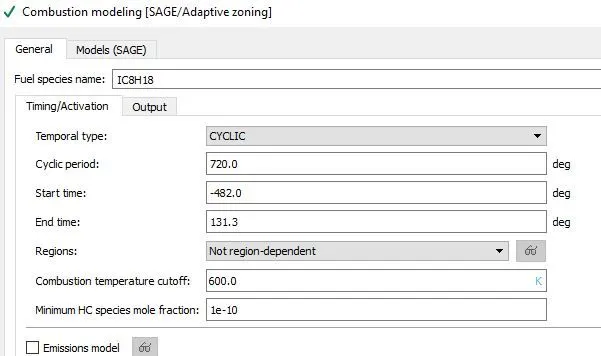
Various combustion models have been developed to simulate a wide variety of combustion phenomena in both spark-ignited (SI) and compression (CI) engines, including spark and auto ignition, laminar and turbulent combustion, premixed, non-premixed and stratified-charge combustion, kinetics and mixing-controlled combustion, and flame propagation combustion. For CI engines, combustion modeling also must resolve two steps: low-temperature chemistry which leads to auto ignition, and the following high-temperature reactions which contribute most of the heat release.
Since combustion in DI engines is turbulent and many turbulent combustion models with different levels of complexity have been proposed for engines applications, including models based on RANS and LES turbulence models. However, since RANS models, specifically the k- model and its variants, are the most commonly used turbulence models at present. In general, there are two ways to describe the combustion process in engine cylinders. One is to use a combustion sub-model to describe the overall combustion characteristics (i.e., flame propagation, reaction rates, and so on) of a combustion process. Combustion models such as mixing-controlled combustion models, flamelet models, and probability density function (PDF) models belong to this category. The other way is to use a detailed reaction mechanism which describes the complex reaction pathways and reaction rates of the important chemical reactions involved in the combustion process and solve for the rate of change of each species in the mechanism.
Before describing the models, two variables which are used in these models are introduced. The first is the mixture fraction (Z) and the second is the reaction progress variable (c). The mixture fraction quantifies the local mass fraction of materials that originate from the reactant fuel. It is mostly used in the analysis and modeling of non-premixed reacting systems. For premixed combustion systems, a reaction progress variable is used. The progress variable increases from zero in the unburned reactants to unity in the burned products. The calculation of the progress variable can be associated with either the mass fraction of a specific species (combustion products) or temperature.
CONVERGE offers two different methods for modeling the ignition and combustion processes. The first method uses separate models for ignition and combustion. These models
are based on the Shell ignition model and the Characteristic Time Combustion model, and this method is relatively computationally inexpensive. The second approach, described in the SAGE detailed chemical kinetics solver section, considers much of the chemistry taking place in combustion applications. Although the runtime using detailed chemistry can be significantly longer than with the first approach, the accuracy of the simulation may be greatly enhanced with the inclusion of detailed chemistry. Nonetheless, there is still often a need for the rapid turnaround time that can be achieved when the simpler models are used.
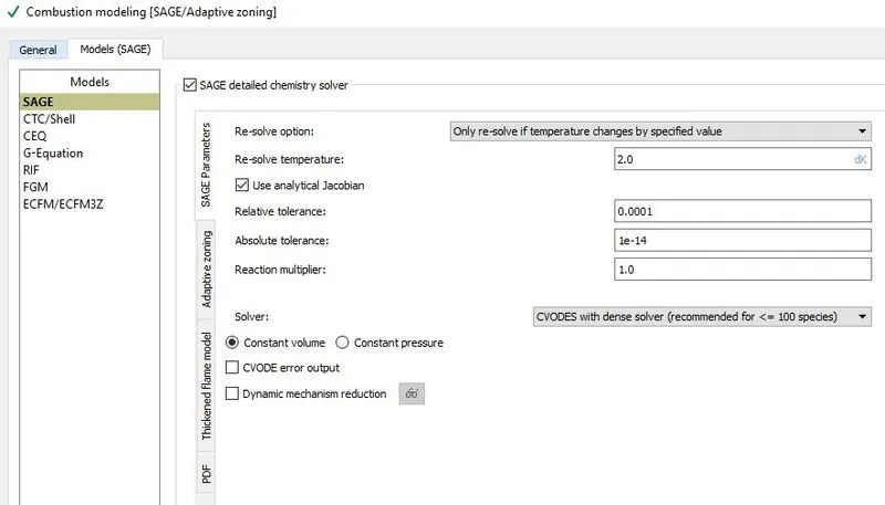
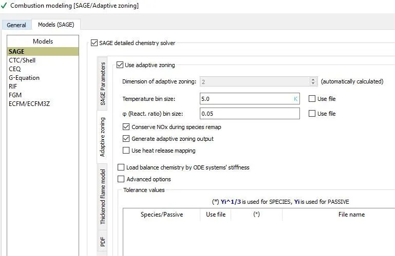
CONVERGE contains the SAGE detailed chemical kinetics solver which models detailed chemical kinetics via a set of CHEMKIN-formatted input files. To solve the systems of ordinary differential equations (ODEs), SAGE uses the CVODE solver, which is part of the SUNDIALS (SUite of Nonlinear and DIfferential/ALgebraic equation Solvers) package.
A chemical reaction mechanism is a set of elementary reactions that describe an overall chemical reaction. The combustion of different fuels can be modeled by changing the mechanism (e.g., there are mechanisms for isooctane, gasoline, n-heptane, natural gas, etc.). SAGE calculates the reaction rates for each elementary reaction while the CFD solver solves the transport equations. Given an accurate mechanism, SAGE (in addition to AMR) can be used for modeling many combustion regimes (ignition, premixed, mixing-controlled). You can use SAGE to model either constant-volume or constant-pressure combustion. Note that SAGE consistently uses CGS units for all calculations.
PROCEDURE:
We already have successfully done surface preparation and boundary flagging of PFI geometry.
Fixed Embedding
Use fixed embedding to refine the grid at specific locations in the domain where a finer resolution is critical to the accuracy of the solution. For example, when simulating sprays, you can add an area of fixed embedding by the nozzle to resolve the complex flow behavior. Fixed embedding allows the rest of the grid to remain coarse to minimize simulation time. For each fixed embedding, you must specify an embedding scale that indicates how CONVERGE will refine the grid in that location.
Depending on the flow taking place, we may require that the flow at some region is more accuracte and at some region ia more approximate. This can be done by varying the mesh element sizes in the region. The embedding option in CFD converge does this work of creating finer mesh at the mentioned location. The refinement is based on the scale and number of embed layers. If the base mesh created has cubic elements of size 'E' mm then the scale of n means the elements in the refinement region will be of size E2n">E2nE2nmm. This means that if the base mesh has elements of size 4mm then elements of scale 1,2,3,4,5 will have elements of size 2,1,0.5,0.25,0.125mm respectively. With each element scale there is 8 times increase in total cell count. This happens because the elements are divided in size by 2 in all directions. Fixed embedding is provided near valve angles as the space between the valve angle and valve seat is very small and base grid with 0.004 m grid size will give inaccurate results.
Fixed embdding is provided to refine the specific areas and capture the combustion details and calculate them properly. cylinderical shape type embedding is provided on the cylinder to make them finer as compared to the base grid.
Adaptive mesh refinement
The adaptive mesh refinement is a method of adopting the accuracy of the solution within a certain sensitive or turbulent region of simulation, dynamically and during the time the solution is being calculated. When curvature exceeds a particular value, the cell will be embedded. we used this formula for the AMR
Size of the cell in scaled grid = (Size of cell in base grid) / 2^(amr_embed_temp_scale)
for exmple
Base grid = 0.8m
amr_embed_temp_scale = 2
size of cell in base grid = 0.8/2^2 =0.8/4=0.2m
The fixed embedding setting is preferred when the refinement is needed in the complete region or complete boundary area. When the refinement is to be done on the solution of flow equations, the refinement technique is called AMR. The AMR monitors the solution and based on the curvature (second degree of rate of change) of a variable, the mesh is refined. There are two methods to use AMR: Sub-grid scale method and value-based method. In the value-based method, the value of a solution is specified. If the value is more/less than specified, the mesh is refined.
PROCEDURE:
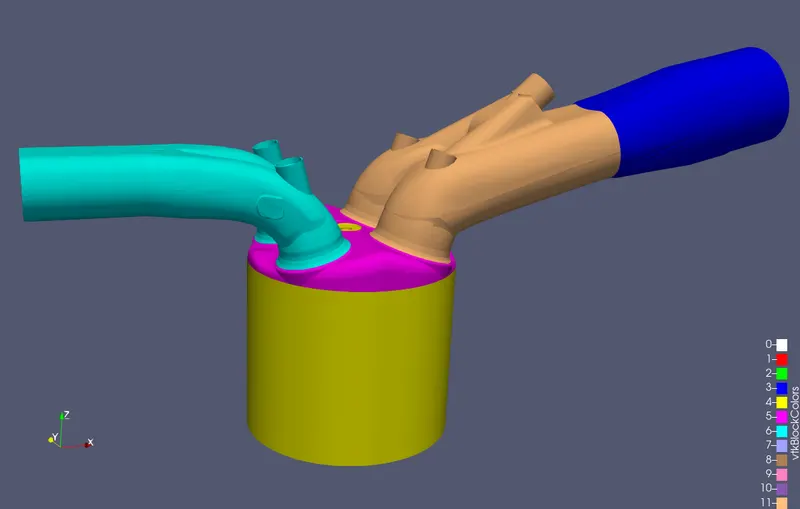
The CAD model was imported into CONVERGE STUDIO and a topological cleanup was performed after diagnosing the model to find the errors.
Geometry
Piston (Piston Head)
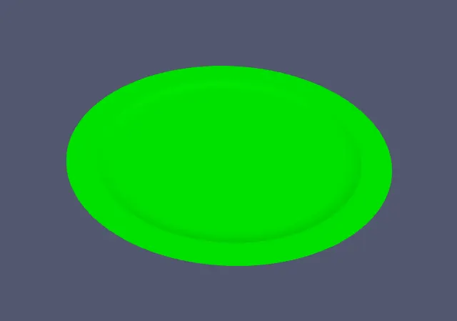
Liner

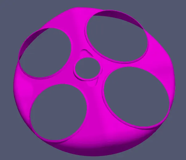
Cylinder Head
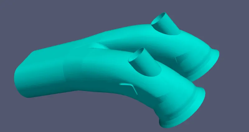
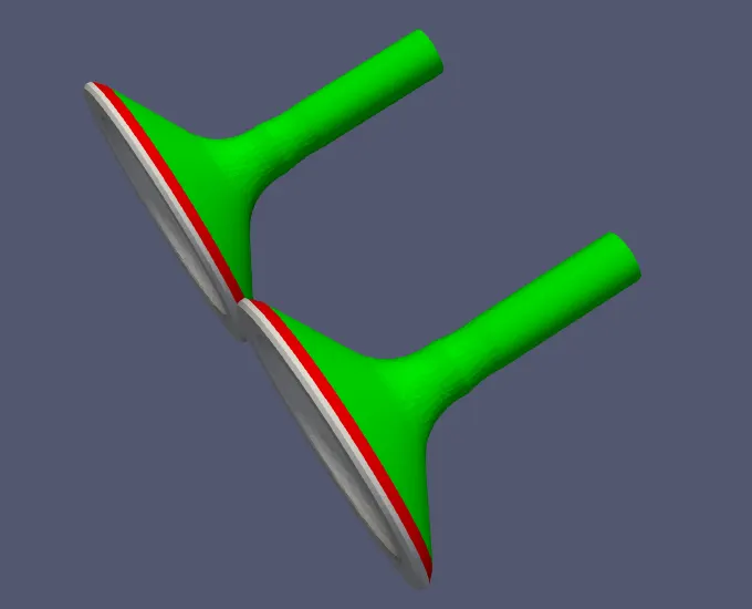
Exhaust Port
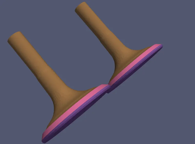
Exhaust Valve
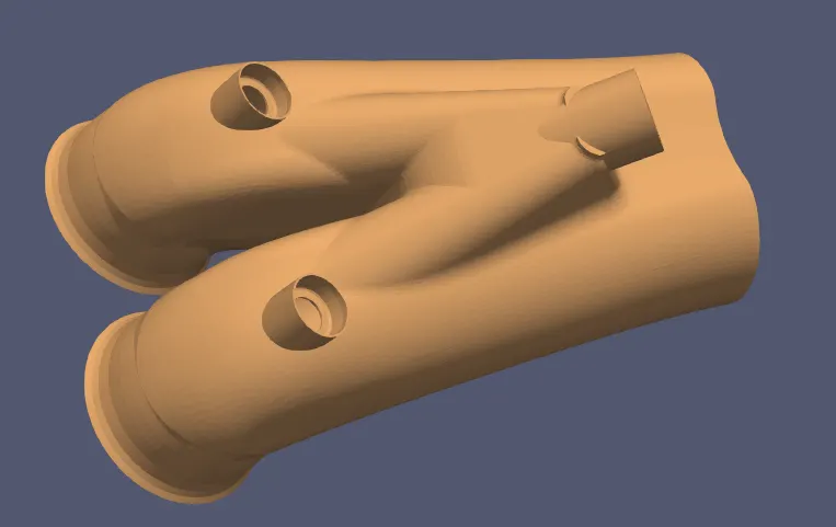
Intake port
Intake valve
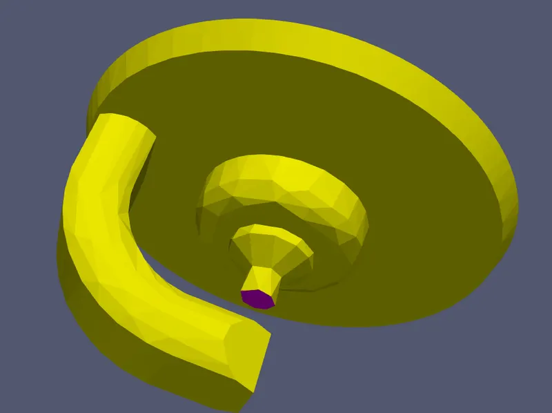
Spark plug
NO HYDRO case setup
Crank angle based
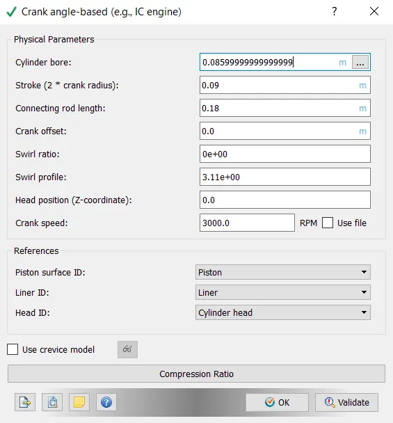
- Real gas (AIR)
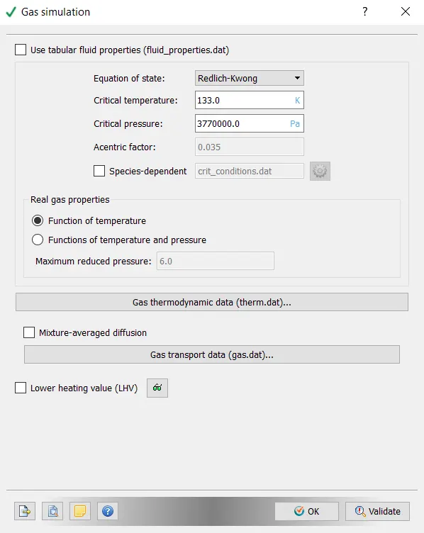
- Reaction Mechanism
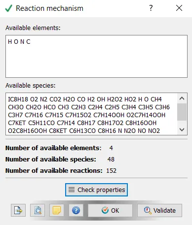
Reaction mechanism is imported, using the provided file "mech.dat"
- Run parameters
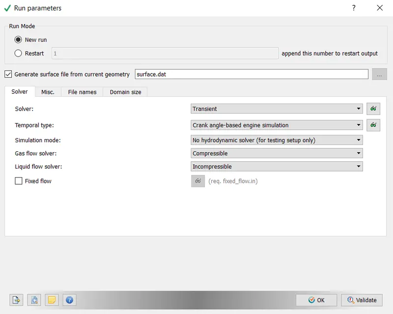
- Simulation time parameters
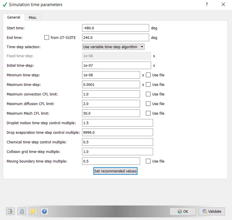
As a time we set crank angle to simulate the whole one cycle of the IC engine.
Boundary Conditions
Piston
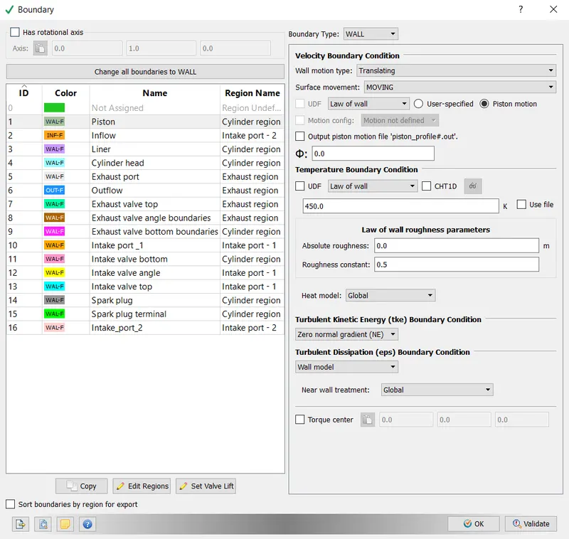
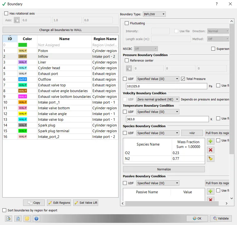
- Inflow
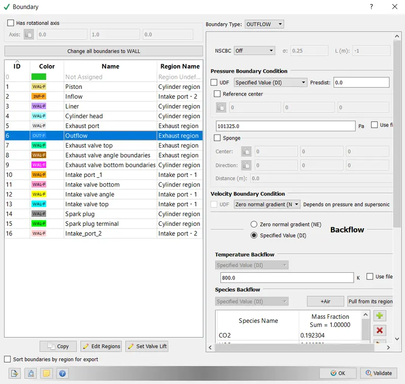
- Outflow
- Intake valve top, angle and bottom
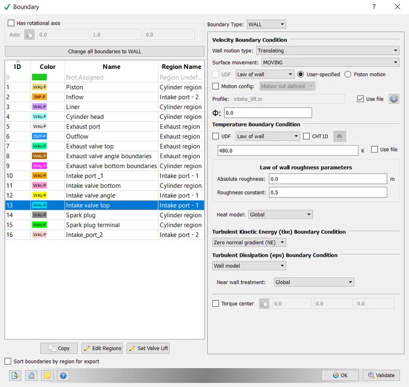
Intake valve top, angle and bottom are different surfaces with the exact same boundary conditions. Valve motion is defined using the provided file "intake_lift.in"
- Exhaust valve top, angle and bottom
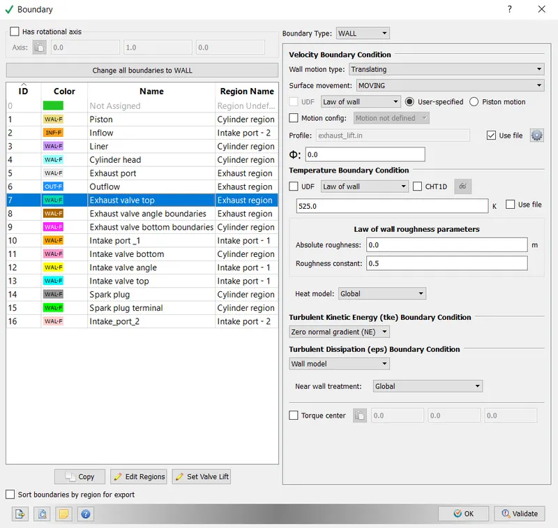
Exhaust valve top, angle and bottom are different surfaces with the exact same boundary conditions. Valve motion is defined using the provided file "exhaust_lift.in".
All other boundaries are the fixed wall boundaries, however the only difference is the Temperature boundary condition.
- Liner - 450K
- Cylinder head - 450K
- Exhaust port - 500K
- Intake port_1 - 425K
- Intake port_2 - 425K
- Spark plug - 550K
- Spurk plug terminal - 600K
As a fuel we use liquid Isooctane (IC8H18)
- Stoichiometric calculatior
For the combustion of our fuel we have an equation 1.
1)
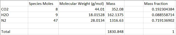
- Initial Conditions and Events
Cylinder region
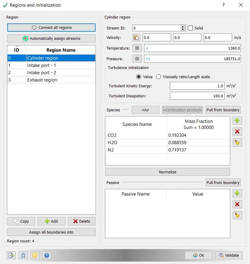
Intake port - 1
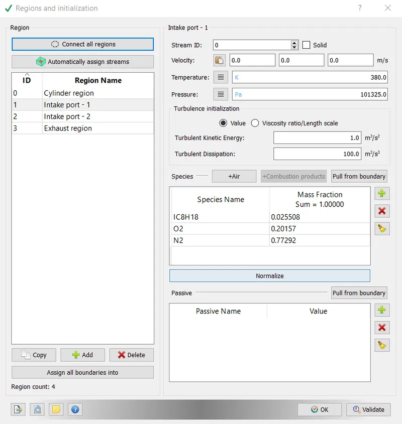
Intake port - 2
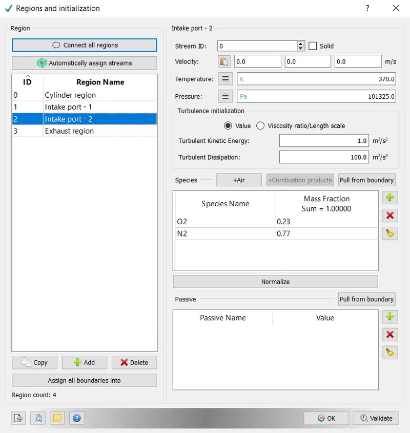
Exhaust region
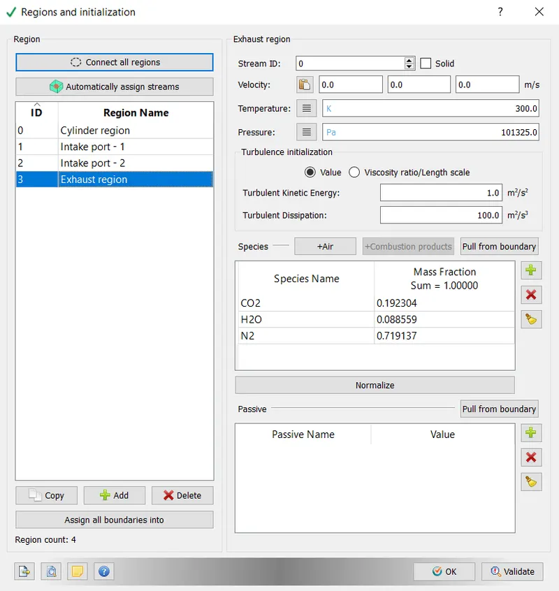
- Events
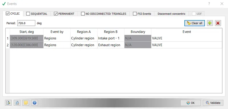
In the event above we see that cylinder ragion is connected with the Intake port - 1 and Exhaust region during the spacific range of crank angle.
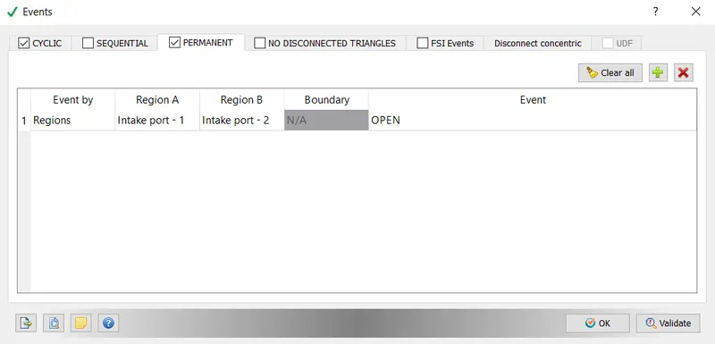
Intake port - 1 and Intake port - 2 are always open to each other.
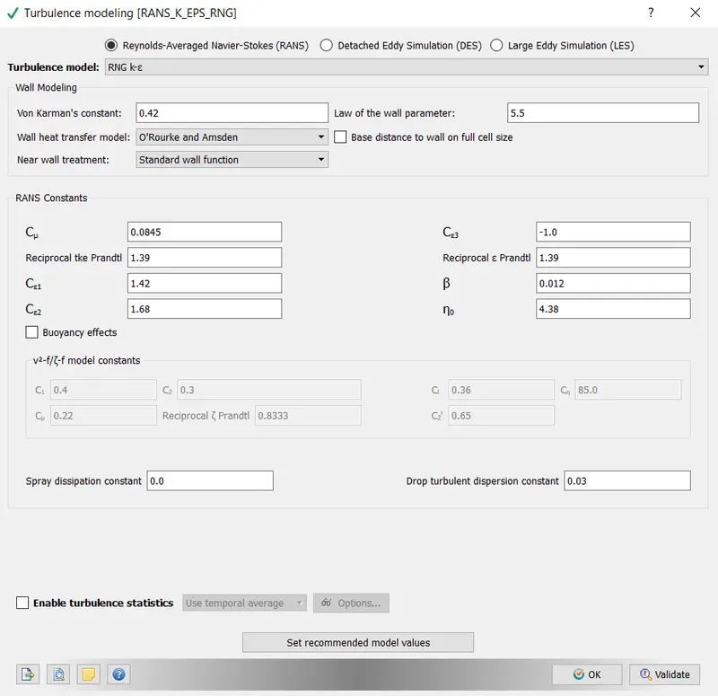
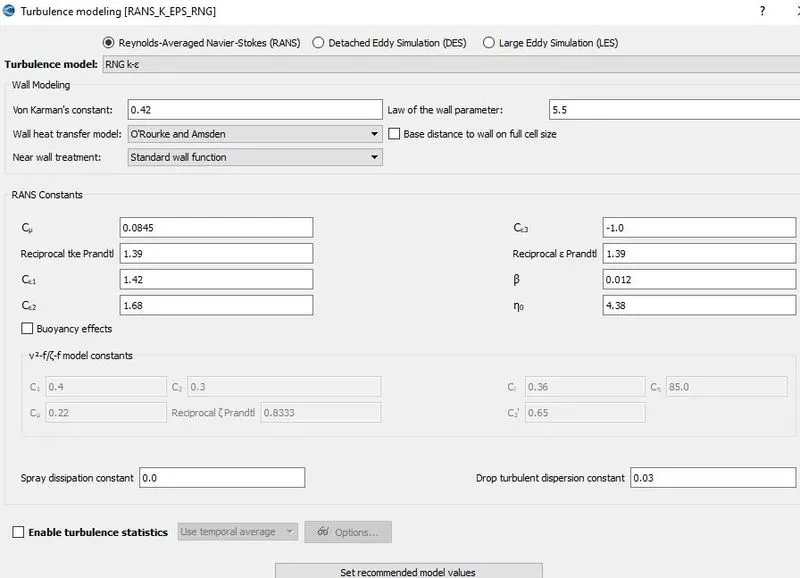
- Turbulence model
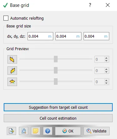
- Base grid
FULL-HYDRO CASE SETUP
Mesh setting
- We have use the 0.004m(4mm) as the base mesh griding.
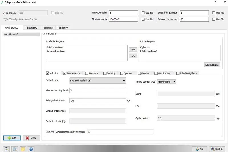
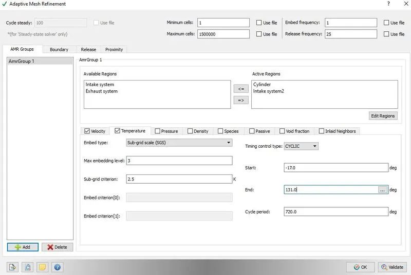
In the spark ignition the main role quantity are temperature and velocity. In the below i shown the velocity and temperature AMR settings.
Embed type = Sub-grid scale(to super quantifying the mesh)
Max embed level = 3
Timing control type = permanent (constant velocity at each crank angle)
Max cells = 2000000( cell sizes increases means the simulation time quite low and slightly decreases the accuracy)
Adaptive Mesh Refinement
Velocity and temperature based grid refinement are performing on cylinder and intake port(near the cylinder region.
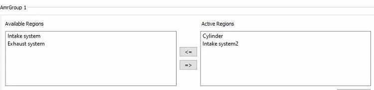
Velocity based AMR
Temperature based AMR
Fixed Embedding
In the fixed embedding we do the following settings.
|
Sr No. |
Embedding name |
Embedding type |
Embedding on |
Embedding mode |
Scale (Element size) |
Embed layers |
Radius 1 at coordinate-1 |
Radius 1 at coordinate-2 |
Cyclic details |
|
|
1 |
Intake valve angle |
Boundary |
Intake valve angle |
Permanent |
3(0.5 mm) |
2 |
||||
|
2 |
Exhaust valve angle |
Boundary |
Exhaust valve angle |
Permanent |
2(1 mm) |
2 |
||||
|
3 |
Big cylinder embedding |
Cylinder |
Volume |
Permanent |
1(4 mm) |
- |
||||
|
4 |
Small cylinder embedding |
Cylinder |
Volume |
Permanent |
2(1 mm) |
- |
0.06m at (0,0,0.1) |
0.06m at (0,0,-0.2) |
||
|
5 |
Spherical embedding |
Sphere |
Volume |
cyclic |
5(0.125 mm) |
- |
0.001 m at (-0.003, 0,0.0091) |
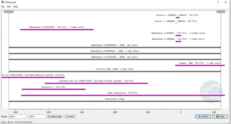
From -16 deg to 0 deg (720 deg period) |
||
|
6 |
Large sphere |
Sphere |
Volume |
cyclic |
4(0.25 mm) |
- |
0.003 m at (-0.003, 0,0.0091) |
From -16 deg to 0 deg (720 deg period) |
||
|
7 |
Injector embedding |
Injector |
Volume |
cyclic |
4(0.25 mm) |
- |
Radius1= 0.002, Radius2= 0.004, length = 0.2 |
From -485 deg to -265 deg(720 deg period) |
||
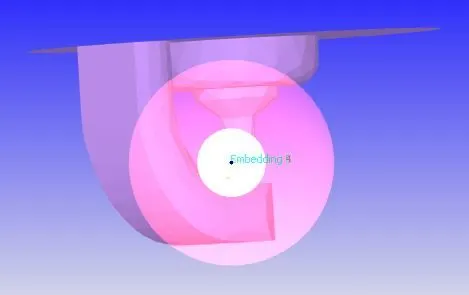
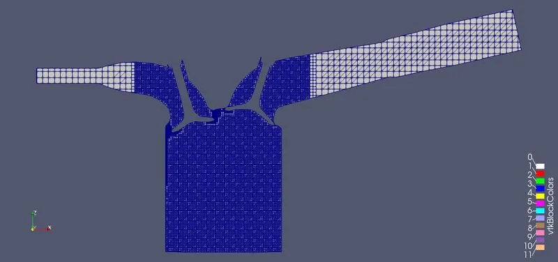
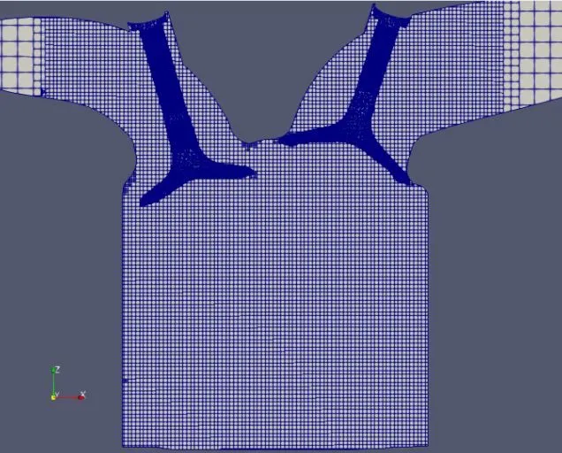
- Embedded regions are also shown in the following figures.
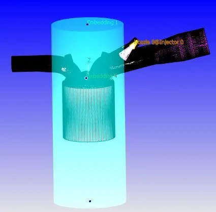
Spray modeling:
In the general tab we do the following setting.
- Parcel distribution: we choose the option distribute parcels evenly throughout cone.
- Turbulent dispersion : we choose the O'Rourke model.
- Droplet evaporation : We choose the Frossling model.
- Evaporation Source: We choose the option source all base parcel species.
- In the spray penetration tab, we choose the 0.95 for the liquid fuel mass fraction.
- Bin size for vapor penetrtion = 0.001
- Fuel mass fraction for calculating vapor penetration = 0.001
- Mass diffusivity constant: We use the iso-octane default values.
In the collision/Breakup/Drag, we do the following settings.
- Collision model: Choose the NTC-collision model
- Collision outcomes: Post collision outcomes
- Level of collision mesh : 2
- Drop drag model: Dynamic drop drag model
In the wall interaction we do the following settings.
- Spray wall interaction model: Wall film
- Film spalsh model: O'Rourke
In the injectors tab, we do the following settings.
- Injected species: IC8H18
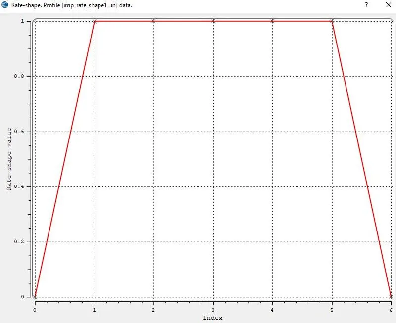
- Rate shape : profile as shown in the below figure.
- Models: Kelvin Helmolthz model
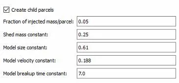
- Child parcels:
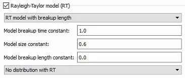
- Rayleigh Taylor Model
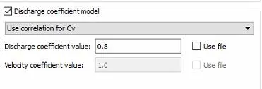
- Discharge coefficients
- In the Mass,time and temperature we do the following settings.
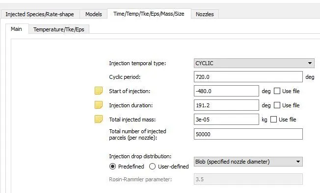
Fuel mass calculation
RPM = 3000
RPS = RPM/60 = 3000/60 = 50
DPS = RPS * 360 = 50 * 360 = 18000
Time per degree = 1/DPS = 1/18000 = 0.000055555 = 5.55e-5
Time per 720 degree = Time per degree *720 = 5.55r-5 * 720 = 0.004
Total flow rate = 7.5e-04 kg/s
Fuel mass per cycle = Total flow rate * Time per 720 degree = (7.5e-04)* 0.004 = 3e-05
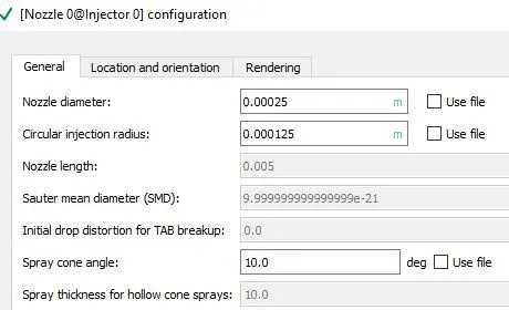
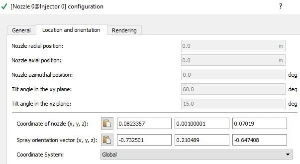
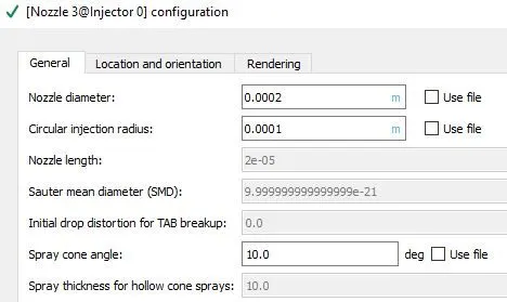
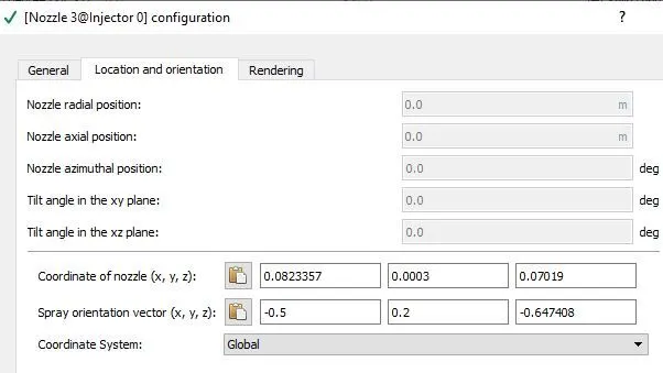
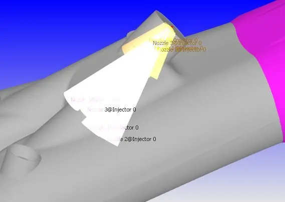
- We choose the four nozzles and do the following settings.
Nozzle_0 configuration
Nozzle_1 configuration
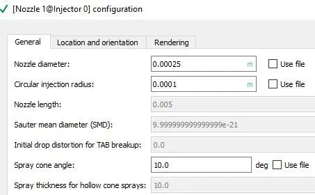
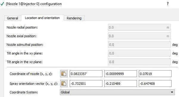
Nozzle_2 configuration
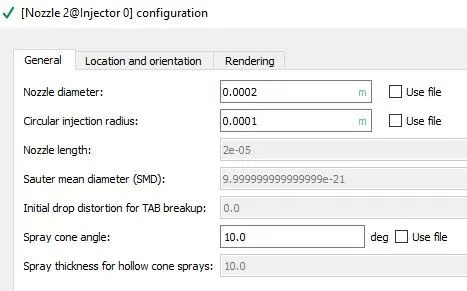
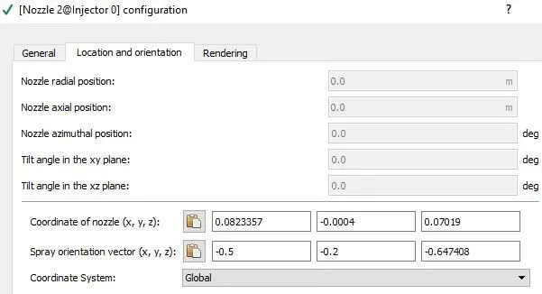
Nozzle_3 configuration
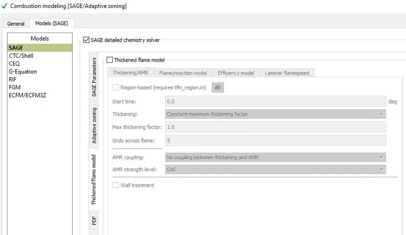
Combustion Modeling
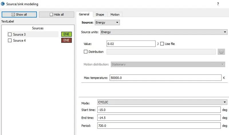
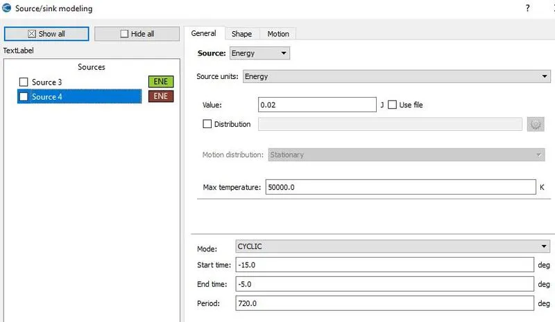
Source Modeling
Source-1
Source-2
Turbulence Modeling:
Mesh
RESULTS:
Volume
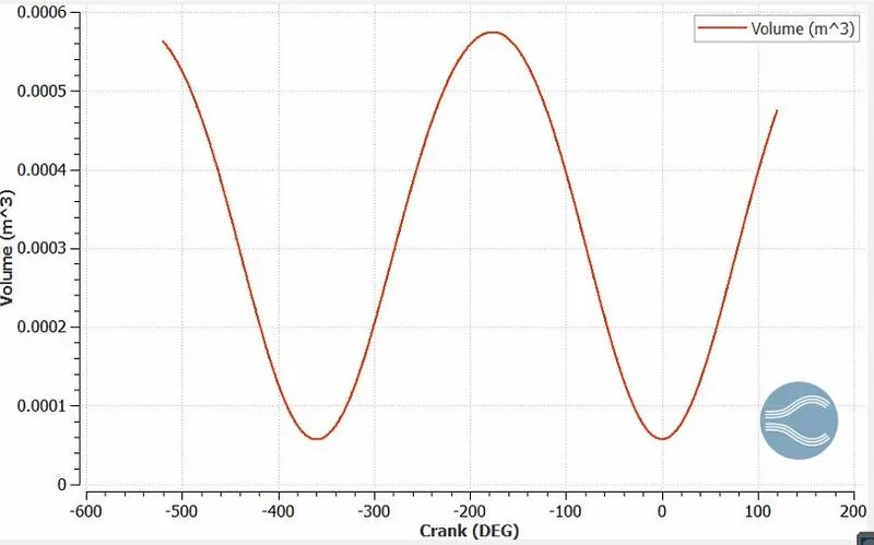
The volume Vs crank angle graph plotted in the cylinder region of the engine. It appears close to sine but its not purely a sine wave. It gives the distance of volume depending on the crank angle.
Pressure
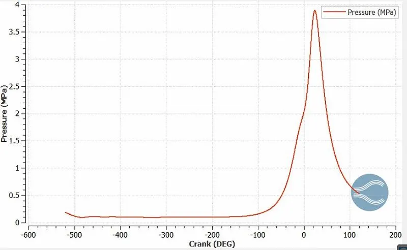
The cylinder contains different values at different strokes of th cylinder, the highest of which is achieved during the end of the compression stroke and it decreases as the combustion and expansion take place. At the end of the compression stroke, the spark plug ignites the air-fuel mixture, creating very high cylinder pressure which rises very quickly. In expansion stroke engine generates power, as it forces the piston down. As the piston goes down, the cylinder volume increases which reduce the cylinder pressure right after it. The peak pressure obtained in this cylinder 3.8MPa.
In the above plot at the 40 degree crank angle combustion has started and then expansion stroke has been started.
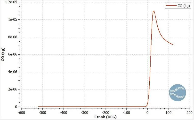
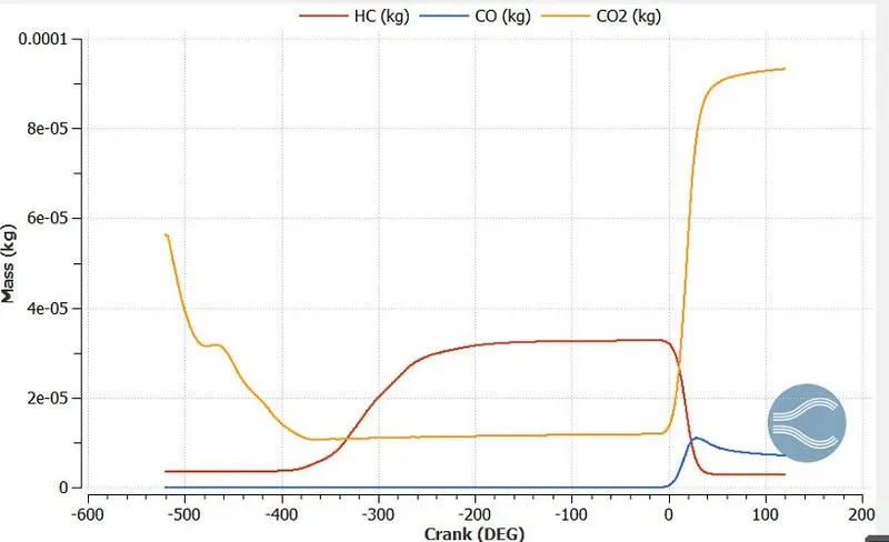
In the above plot we can easily see that the during the exhaust, intake and compression stroke carbon monoxide did not increase but in the power stroke sudden increase of CO is occur. When the power stroke fuel burnt and vapours are created and some unburnt carbon are also extracted. But the quantity of unburnt gases are very small than the burnt gases.
At the 20 degree crank angle CO increases.
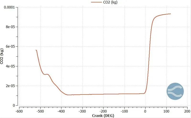
In the above plot first stroke is the exhaust stroke, second is intake, third is compression stroke and last stroke is the power stroke. We can easily observe that during the exhaust the rate of carbon dioxide is decreases and it shows constant behaviour till power stroke stroke and CO2 goes to increase after the power stroke.
Mean temperature
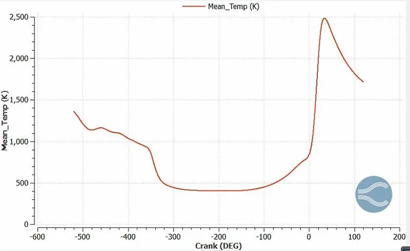
Temperature and pressure are directly proportional to each other, when pressure increases variation in temperature are also occur. In the above plot we can easily observe that engine remains a minimun temperature which is 500K till the start of combustion in the cylinder region. When the power strokes occurs temperature increases because of the reaction of fuel which is being ignited. Mean temperature inside the cylinder region reached is 2483.5. The mean temperature is maximum at the point when the integrated heat release is close to its maximum value, i.e. the entire heat energy is released. It is also the point where there is maximum pressure in the cylinder.
Heat Release Rate
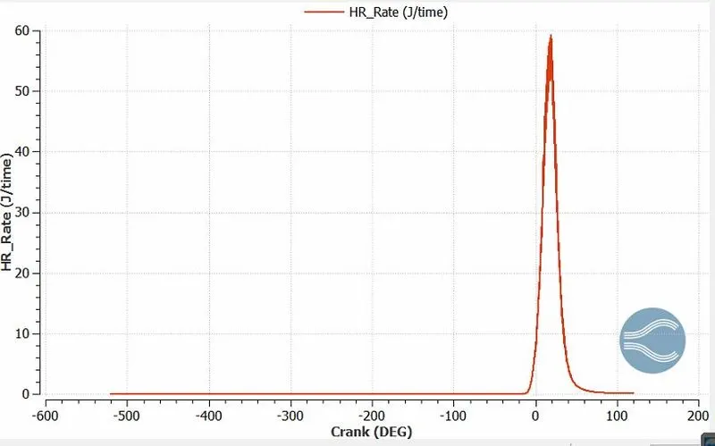
We can easily observe that during the exhaust, intake and compression stroke HR_rate is constant and Heat release rate increases in the power stroke stroke and after that it is going to decrease.
Integrated heat release rate
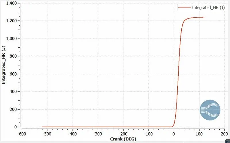
We can easily observe that during the exhaust, intake and compression stroke integrated_HR is constant and Heat release rate increases in the power stroke.
Mass Injected
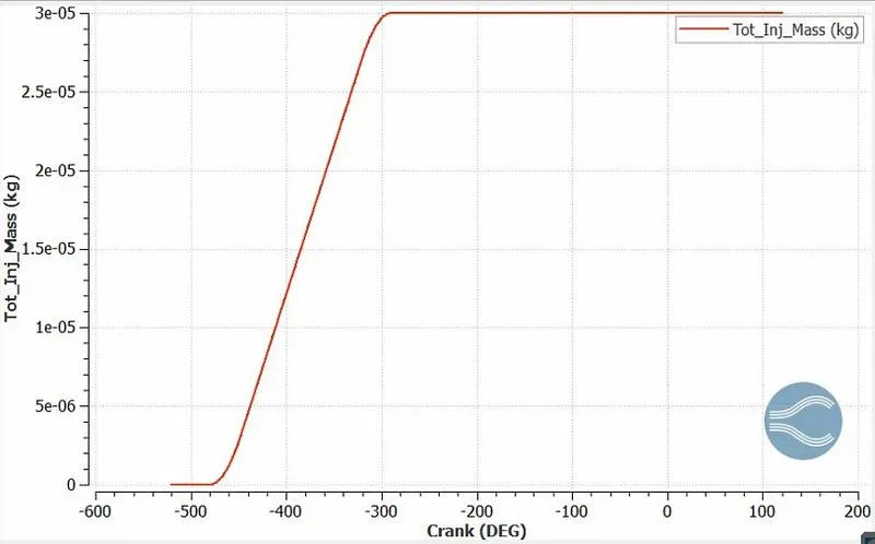
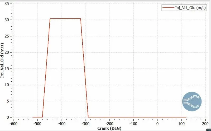
Injection Velocity
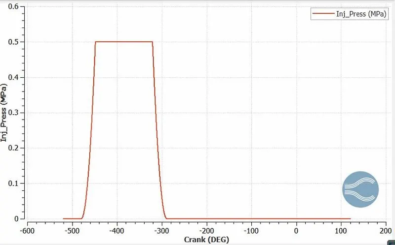
Injection pessure
Species Mass
Spray penetration length
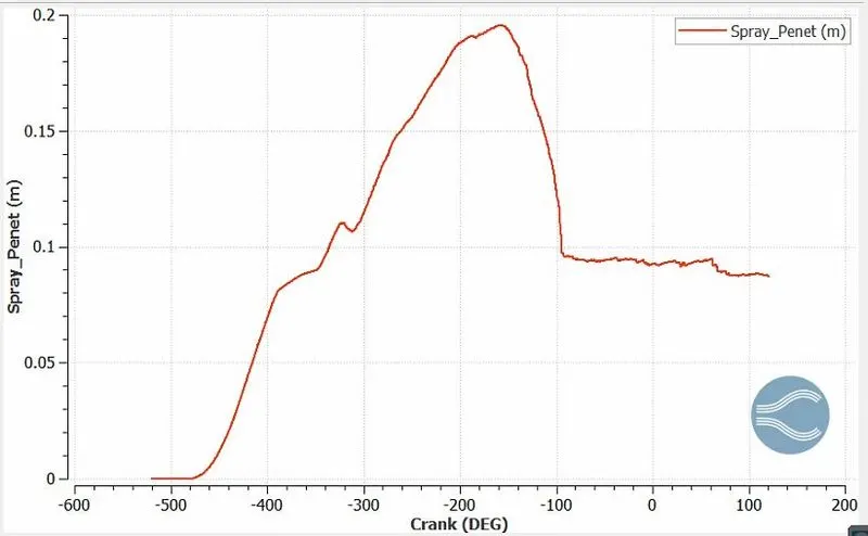
In the above spray penetration graph, we can easily see that we obtain the maximum length at -150 crank angle degree.
NOx
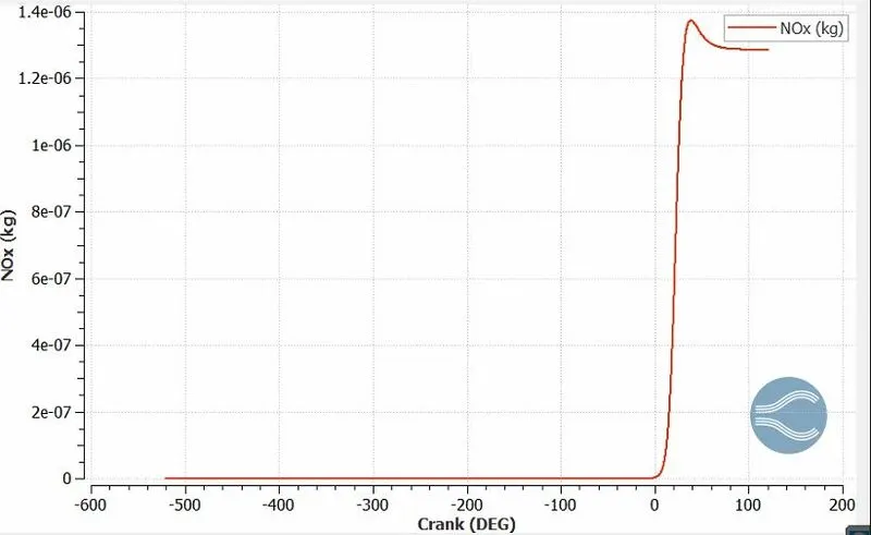
In the above plot we can also see that the rate of NOx formation is high at 0 degree crank when power stroke start and it is going to decrease at a 60 degree crank angle.
Smd
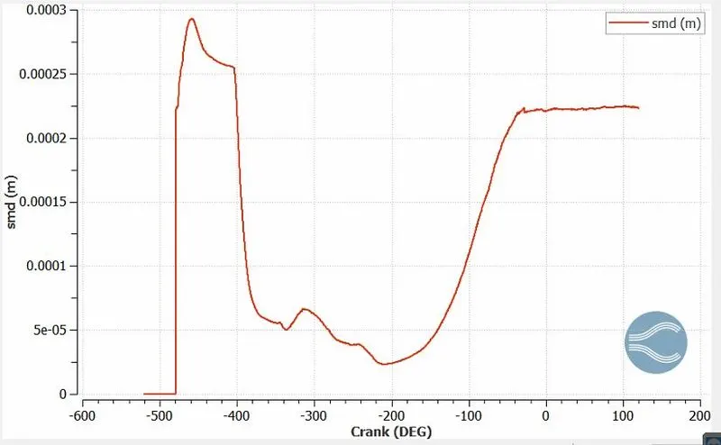
Spray parcel drop
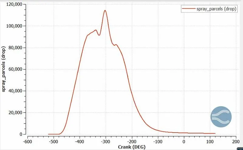
Species parcels drop
Liquid spray drop plot gives the no of lagrangian parcels active in the domain. According to model assumption we inject the drops which is significantly equal to the nozzle hole initially and then it is going to disintegrate. This plot tells about the number of fuel drops and that are created during the spray of fuel into the combustion chamber. The drops are disintegrate due to vaporization. In the above we can observe that after the combustion takes place in the end of the graph shows that amount of drops which are leftover is the unburned hydrocarbon. From that we can also observe that how many fuel have been burned and how many is left.
Total parcels
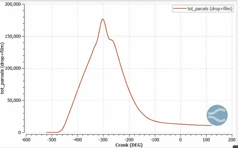
Ca">CaCa
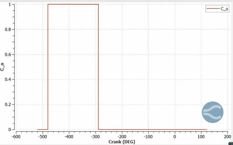
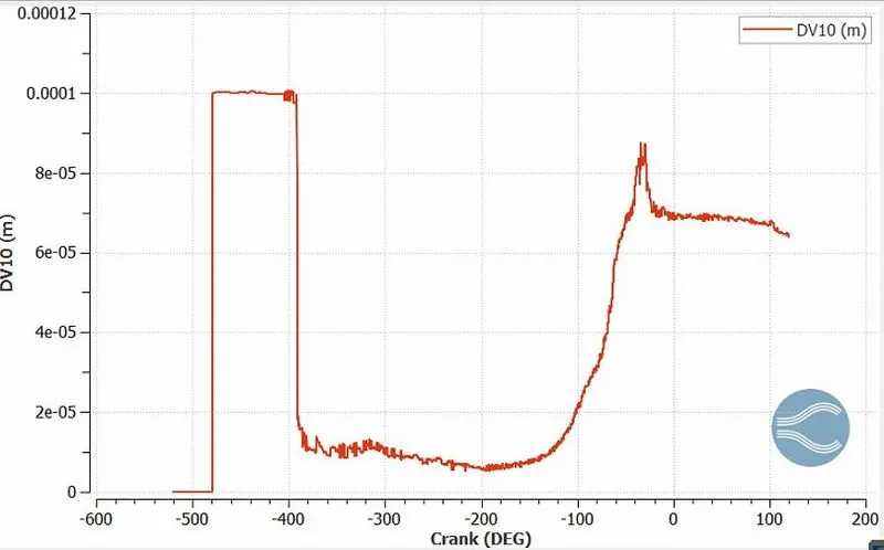
DV10
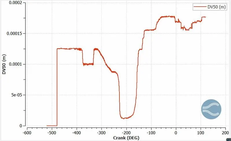
DV50
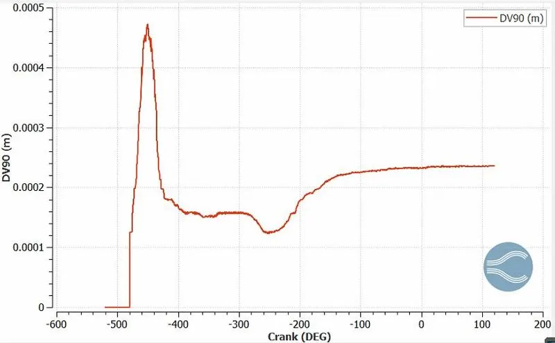
DV90
Timing map
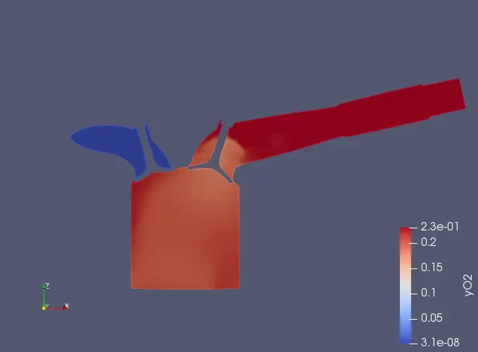
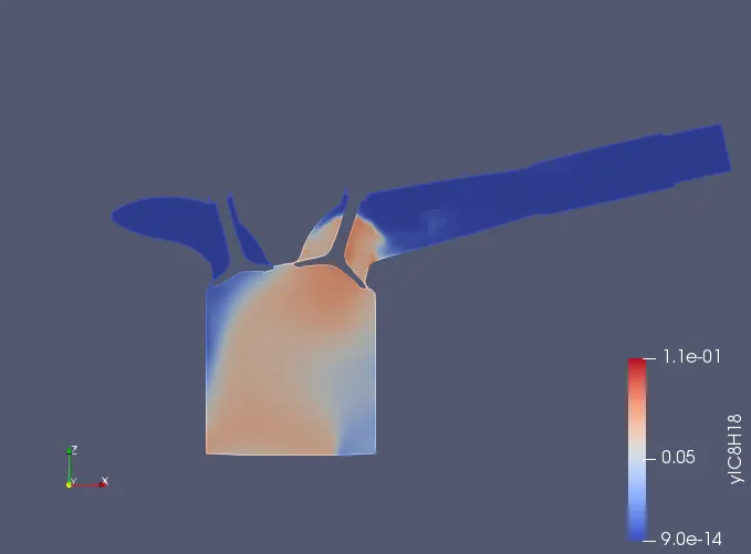
CONCLUSION:
Calculation of compression ratio
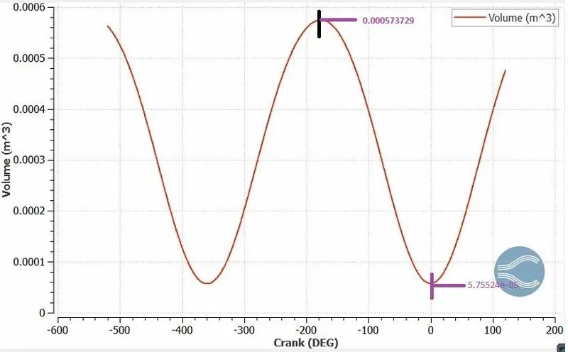
The compression ratio of an engine is the total volume of cylinder to clearance volume of cylinder. The maximum volume is 0.000573729 and minimum volume is 0.0000575524. So the calculated compression ration is 9.968811.
By loading the .thermo and engine.in file we got the following values
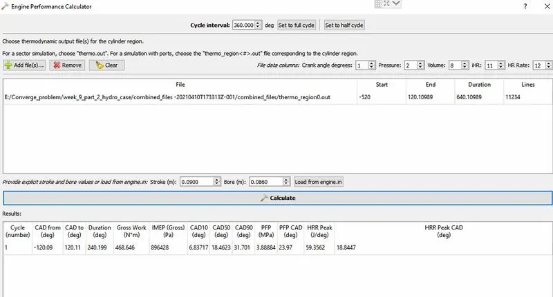
These values are used to calculate the different data for engine.
Calculation of combustion efficiency
|
Pfi combustion calculation eta_c = frac{IHR}{m times LCV_(fuel) Where IHR is the integrated heat release rate and we obtained from the IHR graph. LCV is the lower calorific value IHR = 1240.95 LCV of Iso-octane = 44400 KJ/kg m = 3e-05kg ηc=1240.7244400×3e-05">ηc=1240.72/(44400×3e−05) 0.9315 or 93.15% |
Caculation of power and torque
|
The result of engine performance is calculated from tool of Converge CFD. It gave the following output
Power calculation for PFI using engine calculator Work = 468.646 Duration = 240.199 Power =work/sec RPM = 3000 RPS = 50 1 rotation = 360 degree DPS = 50*360 = 18000 Time(sec) = 240.199/18000 = 0.0133443889 Power = 468.646/0.0133443889 = 35119.330192782 KJ, 35.119KW Torque calculation Power = 2*pi*N*T Torque(T) = Power/(2*Pi*N) Where N- rev/sec T-Torque (N.m) Power – KW N = 50 rev/s Power = 35119.330192782 KJ, 35.119KW Torque = 111.881 |
Wall heat transfer model
It is known that heat transfer in diesel engines affects engine efficiency and emission. An increase of heat transfer to the combustion chamber walls is lower the in-cylinder pressure and the average gas temperature and this reduces the work per cycle transferred to the piston. Thus, the magnitude of engine heat transfer is strongly dependent on engine efficiency. The changes in the gas temperature due to heat loss through the combustion chambers also have an impact on the pollutant emission formation. A higher in-cylinder temperature promotes the NOx emissions and the lower in-cylinder temperature causes the particulates during the exhaust. Since the engine heat transfer is important, the accurate predicted engine heat transfer results are needed. There are many previous experimental and numerical studies on engine heat transfer reported in the literature. The numerical modelling of engine wall heat transfer was researched and improved over the last few decades.
The importance of heat transfer for engine design and optimization has been highlighted by several authors in literature. The reasons are the accurate calculation of performance
parameters, fuel consumption and emissions. Still nowadays heat transfer and wall temperature measurements are not always an option for internal combustion engine design and
optimization, this way the models for this kind of application are the only alternative in many situations for estimation/ calculation of heat transfer and wall temperature. Historically, the frst model for engine heat transfer was presented by Nusselt (1923), based on experiments in a spherical bomb. In this section, the models presented in literature for estimation/calculation of engine heat transfer and wall temperature are reviewed. These models are organized in three heat transfer modelling approaches as follows:
1. Gas to wall heat transfer;
2. Wall to wall heat transfer;
3. Wall to liquid heat transfer.
Gas to wall heat transfer is the modelling approach for the heat exchange between gases and walls in cylinder, intake and exhaust engine regions. Most of the papers in literature
addressing heat transfer inside internal combustion engines refers exclusively to this heat transfer approach. Wall to wall heat transfer approaches are those used to calculate heat
fuxes inside engine parts (head, piston, valves, block, etc.). The third modelling approach is dedicated to calculate heat fux to coolant and lubricating oil.
The combination of gas to wall, wall to wall and wall to liquid approaches is required to estimate/calculate engine internal wall surface temperature, inside the cylinder, ports
and ducts, and specially for valves and piston. For any kind of engine, using those approaches means working with convection-conduction problems, although in diesel engines, it
can involve radiation in some cases (very sooting fames).
The use of the three heat transfer approaches coupled can be found in some applications, for example in order to perform CHT (conjugate heat transfer) analysis where those
heat transfer approaches are coupled to any engine thermodynamic model.
Why can't we Predict the wall temperature from the CFD simulation
In real life, some part of the heat due to combustion is realeased from the cylinder walls. This heat transfer takes place due to all modes of heat transfer. When more than one heat transfer modes are connsidered in the simulations with solid bodies, the simulation is called a conjugate heat transfer simulation. Simulating the IC engine flow along with CHT simulation would increase computation time. So, instead of simulating the heat transfer through would walls, it is modelled (approximated) using different models like O'Rourke model. In this simulation, O'Rourke model is used as wall heat transfer model. We can't predict wall temperature from CFD simulation without using these models, because the wall heat transfer is only captured by a model or CHT simulation and not CFD simulation.
Generally, the operation of an IC engine is based on chemical reactions taking place during combustion. During the power stroke, the fuel-air mixture gets ignited (in spark ignitio engn) by the spark plug and chemical reactions take place inside the combustion chamber. These reactions raise the temperature inside the chamber and force the piston to expand. During this process, there will be an energy interaction between the fluid and solid surface of the IC engine in the form of heat. The heat transfer between the fluid and solid surface takes place generally in two modes: convection and radiation. In general case CFD simulation, the Navier stokes equation is solved to get the results of the fluid flow.
For the PFI engine simulation, it takes a lot of time to compute the case as it involves a complex geometry and processes. If we want to capture the heat transfer, especially convection of heat from the fluid to solid surface energy equations should also be solved. This increases the simulation time.
For simulating complex geometries like IC engines, it takes a lot of time for compting the fluid part itself in a transient case along with combustion and reaction mechanism. So it becomes difficult to predict the wall temperature from the CFD simulations as solving of heat transfer along with Navier stokes equation consumes a lot of computation time and power. Wall heat transfer models are used to approximate this case. Basically all the physical models used in a CFD simulations uses some approximation to minimize the computation time. Wall heat transfer models are used if we are focused only on heat transfer giving less importance to fluid motions and reactions. For efficient operation of engine, the walls should be maintained at a certain temperature. This can only be maintain by pumping coolant to take away the excess heat from the cylinder wall.
Significance of ca10, ca50 and ca90
It is the crank angle at 10%, 50% and 90% where fuel is combusted. From these values we can see that the actual change of crank angle with respect to fuel combustion. The physical significance of CA10 is that it is used to identify the start of ignition in a diesel engine, wheres the CA50 indicate the end of premixed combustion and the start of diffusion combustion of fuel used in the engine.