PID Controller
Target:-
- Different type of DC motor Control.
- Usinf the PID controller in a comtroller.
- Using the MATLAB PID tuner.
Objective:-
- In which situations feedforward control of the DC motor fails? Prepare a MATLAB script for feedforward control and test it.
- Assume a plant and controller. Using MATLAB PID controller block verify system response with General Observation for PID gain Consider the below system:-
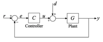
The Plant in this System is `0.3/(s^2 + 0.1s)` - Use MATLAB PID tuner and prepare a table showing PID values with response time and transient behaviour coefficient:-
Blocks required:-
| Sl.No. | Name of the Blocks | Quantities |
| 1. | Constant | 4 |
| 2. | Step response | 1 |
| 3. | Summing point | 1 |
| 4. | PID controller | 1 |
| 5. | Scope | 1 |
| 6. | Transfer Function | 1 |
Theory:-
- Feedback controller:- it helps before the disturbance enters the process the controller takes the action to element the error to be introduced in the system.
- The Advantages are below- :
- Corrective action occurs as soon as the controlled variable deviates from the setpoint, regardless of the source and type of disturbance.
- Feedback control requires minimal knowledge about the process to be controlled; in particular, a mathematical model of the process is not required, although it can be very useful for control system design.
- The ubiquitous PID controller is both versatile and robust. If process conditions change, retuning the controller usually produces satisfactory control
- This controller is not been used in any kind of system because besides this kind of advantages there are many more disadvantages and the disadvantages are more difficult to bypass so it is not been used nowadays
- The Disadvantages are below:
- Complexity as compared to the feedback system.
- Due to various sensor required there should be a correct and complex mathematical model that can help in finding the disturbances.
- Identification of all possible disturbances in the model.
- If there is a slight manipulation in the, mathematically model then the system is fully crashed as there is no method or sensor to sense the requirements.
- It is only reliable in a slow system.
- It cannot cope up with the unmeasured disturbances.
- It is very sensitive to process parameters variation.
- Knowledge of all the possible disturbance should be there.
- A perfect controller can not occur.
- The predictive controller does not occur.
- The controller can be unsatisfactory for the process with large dead times.
- The disturbance variables must be measured online. In many applications, this is not feasible.
- To make effective use of feedforward control, at least an approximate process model should be available. In particular, we need to know how the controlled variable responds to changes in both the disturbance and manipulated variables. The quality of feedforward control depends on the accuracy of the process model.
- Ideal feedforward controllers that are theoretically capable of achieving perfect control may not be physically realizable. Fortunately, practical approximations of these ideal controllers often provide very effective controller.
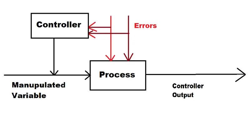
- The Advantages are below- :
- A plant in Control Theory is the combination of Process and actuator. A plant is often referred to with a Transfer Function (commonly in the s-domain), which indicates the relationship between an input signal and the system's output signal without feedback, commonly determined by the system's physical properties. An example would be an actuator with its transfer of the input of the actuator to its physical displacement. The plant still has the same transfer function in a system with feedback, but a control unit and a feedback loop (with their respective transfer functions) are added to the system.
- The proportional term, Kp, is entirely based on the error and that, let's say, double the error would mean doubling Kp (applying proportional force). This, therefore, implies that increasing Kp is a result of the system heading in the wrong direction so Kp is increased to ensure the system goes in the right direction or at least tries to reduce the error as time passes so an increase in Kp would affect the system in such a way to adjust the heading of the system so it stays on the right path.
- The derivative term, Kd, is based on the rate of change of the error so an increase in Kd implies that the rate of change of error has increased over time so double the error would result in double the force. An increase by double the change in the system's heading would take place if the system's heading is doubled in error from the previous feedback result. Kd causes the system to react faster as the error increases.
- An increase in the integral term, Ki, means that the error is increased over time. The integral accounts for the sum of error over time. Even a small increase in the error would increase the integral so the system would have to head in the right direction for an equal amount of time for the integral to balance to zero
- We have to make a table which is consisting of all the information related to rising TIME, OVERSHOOT, SETTLING TIME and STEDY-STATE ERROR w.r.t to all the values of `k_p ,k_d & k_i` and using that values making a transfer function we can see what happens when and how to overcome that.
using the above do all the parameter and tune the PID controller.Types Rise Time Overshoot Settling Time Steady-State Error `k_p` `darr` `uarr` `rarr` `darr` `k_i` `darr` `uarr` `uarr` Eliminate `k_d` `darr` `darr` `darr` - `.^2`The PID Tuner app automatically tunes the gains of a PID controller for a SISO plant to achieve a balance between performance and robustness. You can specify the controller type, such as PI, PID with derivative filter, or two-degree-of-freedom (2-DOF) PID controllers. Analysis plots let you examine controller performance in time and frequency domains. You can interactively refine the performance of the controller to adjust loop bandwidth and phase margin or to favour setpoint tracking or disturbance rejection.
You can use PID Tuner with a plant represented by a numeric LTI model such as a transfer function (
tf) or state-space (ss) model. If you have Simulink® Control Design™ software, you can use PID Tuner to tune a PID Controller or PID Controller (2DOF) block in a Simulink model. If you have System Identification Toolbox™ software, you can use the app to estimate a plant from measured or simulated data and design a controller for the estimated plant`.^2`
Solution:-
- The process is below:-
- Open the Matlab script file and define the physical constants as per your motor rating.
- Then construct the state-space model of the DC motor with two inputs
- Compute with the state-space form to minimize the model order.
- Now plot the angular velocity response to a step-change in voltage
- We can use this simple feedforward control structure to command the angular velocity w to a given value w_ref
- The feedforward gain Kff should be set to the reciprocal of the DC gain from Va to w.
- To evaluate the feedforward design in the face of load disturbances, simulate the response to a step command w_ref=1 with a disturbance Td = -0.1Nm between t=5 and t=10 seconds:
- To enforce zero steady-state error, use integral control of the form
- To determine the gain K, you can use the root locus technique applied to the open-loop 1/s * transfer(Va->w)
- Click on the curves to read the gain values and related info. A reasonable choice here is K = 5. Note that the SISO Design Tool offers an integrated GUI to perform such designs
- In addition to the integral of error, the LQR scheme also uses the state vector x=(i,w) to synthesize the driving voltage Va. The resulting voltage is of the form.
- Or better disturbance rejection, use a cost function that penalizes large integral error, e.g., the cost function
`C = int_0^oo (20q(t)^2 + omega(t)^2 + 0.01V_a(t)^2)dt` The Script File is below R = 2.0; % Ohms
L = 0.5; % Henrys
Km = 0.1; % torque constant
Kb = 0.1; % back emf constant
Kf = 0.2; % Nms
J = 0.02; % kg.m^2/s^2
h1 = tf(Km,[L R]); % armature
h2 = tf(1,[J Kf]); % eqn of motion
dcm = ss(h2) * [h1 , 1]; % w = h2 * (h1*Va + Td)
dcm = feedback(dcm,Kb,1,1); % close back emf loop
stepplot(dcm(1));
Kff = 1/dcgain(dcm(1))
t = 0:0.1:15;
Td = -0.1 * (t>5 & t<10); % load disturbance
u = [ones(size(t)) ; Td]; % w_ref=1 and Td
cl_ff = dcm * diag([Kff,1]); % add feedforward gain
cl_ff.InputName = {'w_ref','Td'};
cl_ff.OutputName = 'w';
h = lsimplot(cl_ff,u,t);
title('Setpoint tracking and disturbance rejection')
legend('cl_ff')
% Annotate plot
line([5,5],[.2,.3]);
line([10,10],[.2,.3]);
text(7.5,.25,{'disturbance','T_d = -0.1Nm'},'vertic','middle','horiz','center','color','r');
h = rlocusplot(tf(1,[1 0]) * dcm(1));
setoptions(h,'FreqUnits','rad/s');
xlim([-15 5]);
ylim([-15 15]);
K = 5;
C = tf(K,[1 0]); % compensator K/s
cl_rloc = feedback(dcm * append(C,1),1,1,1);
h = lsimplot(cl_ff,cl_rloc,u,t);
cl_rloc.InputName = {'w_ref','Td'};
cl_rloc.OutputName = 'w';
title('Setpoint tracking and disturbance rejection')
legend('feedforward','feedback w/ rlocus','Location','NorthWest')
dc_aug = [1 ; tf(1,[1 0])] * dcm(1); % add output w/s to DC motor model
K_lqr = lqry(dc_aug,[1 0;0 20],0.01);
P = augstate(dcm); % inputs:Va,Td outputs:w,x
C = K_lqr * append(tf(1,[1 0]),1,1); % compensator including 1/s
OL = P * append(C,1); % open loop
CL = feedback(OL,eye(3),1:3,1:3); % close feedback loops
cl_lqr = CL(1,[1 4]); % extract transfer (w_ref,Td)->w
bodeplot(cl_ff,cl_rloc,cl_lqr);
h = lsimplot(cl_ff,cl_rloc,cl_lqr,u,t);
title('Setpoint tracking and disturbance rejection')
legend('feedforward','feedback (rlocus)','feedback (LQR)','Location','NorthWest')
- Run the model and observe and comment the observe
- For using the PID controller the process is
- Open the MATLAB
- Now go for the Simulink then get the blocks that are required.
- Put the transfer function on the transfer function block.
- Change the solver configuration to od45 which helps solve the PID controller otherwise, there will be some kind of error.
- Now with the default value use record the observation then
- After the observation use the value of the `k_p , k_i & k_d`
- Keeping the value of the 3 observe the change and find out the difference between with PID and without PID.
- For using the PID tunning method follow these steps:-
- Open a new script file in MATLAB.
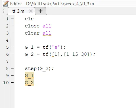
- Type a transfer function with all the necessary codes that are required.
- The transfer function is given as follows
- Run the program
- From the app section run the PID tuner
- Now go for the plant < Import New plant < search for G_2 < change type to PID
- Open the Simulink model by typing the model name at the MATLAB®command prompt.
- To open the block dialogue box, double-click the PID controller block.
- In the block dialogue box, in the Select Tuning Method drop-down list, select Transfer Function Based (PID Tuner App). To open PID Tuner, click Tune.
- PID Tunerautomatically linearizes the plant at the operating point specified by the model initial conditions, as described in what plant does PID tuner see?. If you want to design a controller for a different operating point, see tune at a different operating point.
- PID Tunercomputes an initial compensator design for the linearized plant model using the algorithm described in PID Tuning Algorithm.
- PID Tunerdisplays the closed-loop step reference tracking response for the initial compensator design. For comparison, the display also includes the closed-loop response for the gains specified in the PID controller block, if that closed loop is stable, as shown in the following figure
Observation:-
- Few plots are like this
-
This is the step response. -
The setpoint tracking with the disturbance which is been shown below with the delay in response -
The root locus of the system -
The bode Diagram or the bode plot -
The comparison of both the feedforward and as well as feedback system
-
- There are two kinds of observation one
-
In this, I have not introduced any kind of PID values from which we can found that 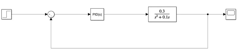
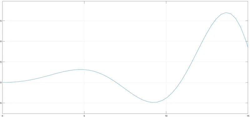
-
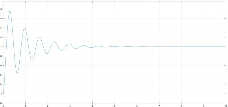
In this I have introduced some values of `k_p ,K_d & K_i` and the values are 300 10 and 350 respectively and due to which the system gets stable quickly and there is 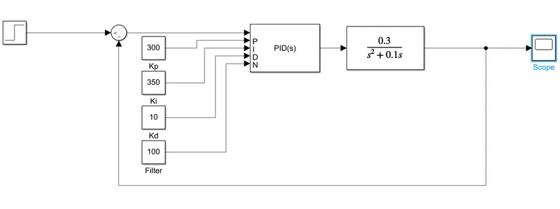
-
- There are 3 observation following by the best one should be taken
-
This one is only taken with the P and D 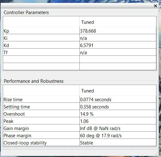
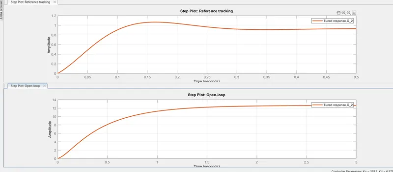
-
This an also a good system but the settling time is not machining and the peak also 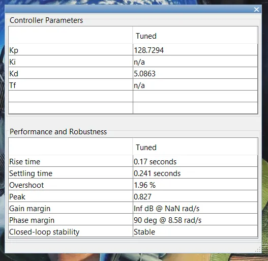
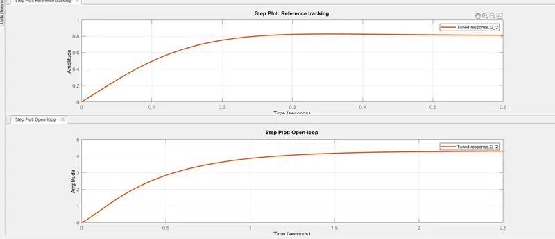
-
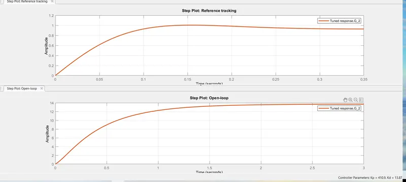
This is the system which I found that is good as per the PID 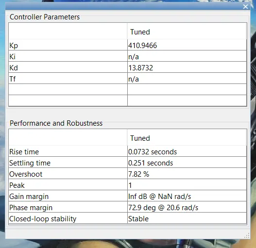
-
Conclusion:-
- Feedforward control is having a lot of disadvantages we can see from the example so we are not using this controller.
- We found that using PID we can make a system stable and good and quick
- Using the PID tuner we got, we can make the system cleaner with the tuner, which helps get the particular tuning using the plant and PID tuner.
Reference:-
- https://in.mathworks.com/help/control/ug/dc-motor-control.html
- https://in.mathworks.com/help/control/ref/pidtuner-app.html