Otto Cycle using engine kinematics

Objective:

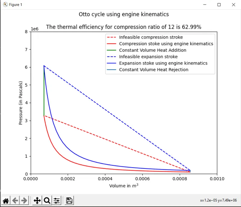
To plot the P-V diagram of the otto cycle while also calculating its thermal efficiency

Problem Statement:

Whether engine kinematics can be effectively used to plot a P-V diagram of the Otto Cycle

Introduction:

The Otto cycle is the ideal cycle for spark-ignition engines, in honor of Nikolaus Otto, who invented it in 1867. In ideal Otto cycles, air-standard assumption is used. The ideal Otto cycle consists of four internal reversible processes:

• 1-2 Isentropic compression
• 2-3 Constant volume heat addition
• 3-4 Isentropic expansion
• 4-1 Constant volume heat rejection

The thermal efficiency of the cycle is given by:

`η= 1-1/(r^(k-1)` - (equation 1)

where

r = compression ratio

k= specific heat ratio

Solution Procedure:

A python program has been made defining the values of compression ratio, length of connecting rod, stroke length, cylinder bore, specific heat ratio & the number of values of instantaneous crank angle

Then using these, we calculate:

`R=(c)/(rad)`

`Vs=(pib^2s)/4`

`Vc=(Vs)/(r-1)`

where,

R= constant

c = connecting rod length in m

rad = crank pin radius in m

Vs = Swept Volume in `m^3`

Vc = Clearance Volume in `m^3`

b = cylinder bore in m

s = stroke length in m

r = compression ratio

Now, to plot the P-V values, we have calculated the values of P,V and T corresponding to each state point from 1-4 using the standard thermodynamic relations. But the path from state point 1-2 and 3-4 are isentropic compression and expansion respectively and hence, to trace that path, I have used to concept of engine kinematics.

The Volume at any point of the compression/expansion stroke is given by:

`V= (Vs)/(r-1)+(Vs)/2[1+R-costheta-(R^2-Sin^2theta)^(1/2)]`

where

V = instantaneous volume corresponding to a certain value of crank angle

Vs = swept volume in `m^3`

r = compression ratio

R = constant defined above

`theta`= instantaneous crank angle

For every value of V, we have calculated the corresponding value of pressure using the thermodynamic relation `PV^k= constant`

We want the value of thermal efficiency, and hence using equation 1, I have calculated its value along with defining an output statement.

Now, after calculating all the requisite values, the final step is to plot these values to a graph to get the P-V diagram. And I have used the matplotlib.pyplot module to make use of the plotting commands and plot the diagram.

The detailed code:

import math
import matplotlib.pyplot as plt


#compression ratio
r=12
#length of connecting rod in meters
c_rod=0.15
#length of stroke in meters
stroke=0.1
#cylinder diameter in meters
bore=0.1
#crank pin radius (stroke length/2) in meters
rad=stroke/2
#constant = connecting rod length/crank pin radius
R=c_rod/rad
#Swept volume of the cylinder from TDC to BDC in m^3
Vs= math.pi*bore*bore*stroke/4
#Clearance volume at TDC in m^3
Vc=Vs/(r-1)
#Specific heat ratio
k=1.4
#no of values of instantaneous crank angle
n=50

#function to calculate instantaneous volume using engine kinematics
def vol_calc(ts,te,n,r,R,Vs):
	V=[]
	dteta=(te-ts)/(n-1)
	for i in range(0,n):
		theta=ts+dteta*i
		a=1+R-math.cos(math.radians(theta))
		b=pow(R*R-pow(math.sin(math.radians(theta)),2),1/2)
		V.append((Vs/(r-1))+(Vs/2)*(a-b))
		
	return(V)

#state point 1:

#Volume in m^3 at the start of compression stroke
V1= Vc+Vs
#Pressure in pascals at the start of compression stroke
P1=101325
#Temperature in K at the start of compression stroke
T1=500

#state point 1-2(compression stroke):

#Volume in m^3 during the compression stroke
v_compression=(vol_calc(180,0,n,r,R,Vs))

#Pressure in pascals during the compression stroke	
p_compression=[]
for v in v_compression:
	#P1*V1^k=P2*V2^k 
	p_compression.append((P1*pow(V1,k))/pow(v,k))
P2=p_compression[-1]

#Temperature in K at the end of compression stroke
#P1*V1/T1=P2*V2/T2
T2=p_compression[-1]*v_compression[-1]*T1/(P1*V1)

#state point3:

#Volume in m^3 at the start of expansion stroke
V3=Vc
#Temperature in K at the start of expansion stroke
T3=2500
#Pressure in pascals at the start of expansion stroke
#P2/T2=P3/T3
P3=p_compression[-1]*T3/T2

#state point 3-4(expansion stroke):

#Volume in m^3 during the expansion stroke
v_expansion=(vol_calc(0,180,n,r,R,Vs))
V4=v_expansion[-1]

#Pressure during the expansion stroke	
p_expansion=[]
for v in v_expansion:
	#P3*V3^k=P4*V4^k 
	p_expansion.append((P3*pow(V3,k))/pow(v,k))
P4=p_expansion[-1]

#calculating thermal efficiency of the cycle
thermal_efficiency= (1-(1/pow(r,k-1)))*100
#rounding efficiency to 2 places
thermal_efficiency=round(thermal_efficiency,2)
print('Thermal Efficiency:',thermal_efficiency,'%')

#plotting the P-V diagram of Otto cycle while also printing the thermal efficiency
plt.plot([V1,v_compression[-1]],[P1,p_compression[-1]],'r--',label='Infeasible compression stroke')
plt.plot(v_compression,p_compression,'r-',label='Compression stoke using engine kinematics')
plt.plot([v_compression[-1],V3],[p_compression[-1],P3],'g-',label='Constant Volume Heat Addition')
plt.plot([V3,v_expansion[-1]],[P3,p_expansion[-1]],'b--',label='Infeasible expansion stroke')
plt.plot(v_expansion,p_expansion,'b-',label='Expansion stoke using engine kinematics')
plt.plot([v_expansion[-1],V1],[p_expansion[-1],P1],'-',label='Constant Volume Heat Rejection')
plt.legend(loc='best')
plt.xlabel('Volume in $m^3$')
plt.ylabel('Pressure (in Pascals)')
plt.title('Otto cycle using engine kinematicsnnThe thermal efficiency for compression ratio of '+str(r)+' is '+str(thermal_efficiency)+'%')
plt.xlim(0,0.001)
plt.ylim(0,8000000)
plt.show()

Results and Discussion:

The diagram successfully replicates the trajectory of an ideal otto cycle by the use of engine kinematics. The thermal efficiency of the cycle under the given set of conditions was found to be 62.99%

References:

1. https://www.engr.colostate.edu/~allan/thermo/page2/page2.html
2. http://www.ecourses.ou.edu/cgi-bin/ebook.cgi?topic=th&chap_sec=08.1&page=theory