Mixing efficiency

OBJECTIVE

• Set up a steady state simulation of a mixing tee and compare the effectiveness for following input conditions using Ansys Fluent

Hot temperature: 36 ^oC = 309.15 K

Cold Temperature: 19 ^oC = 292.15 K

Velocity (hot): 3m/s

Momentum Ratio: velocity at cold inlet/ velocity at hot inlet = 2, 4

Specimen: Short, Long

• Compare K-Epsilon and K-omega turbulence model and select the suitable one for the study.
• Perform mesh independent study for one of the cases.
• Extract following details
• Velocity and Temperature contour plots
• Discuss the effect of length and momentum ratio on the effectiveness

THEORY

There are two RANS based turbulence model

• K-Epsilon and 2) K-omega

K- ε

It is a 2 equation model in CFD to solve the characteristics of turbulent flow. K represents the kinetic energy whereas ε represents the rate of dissipation of turbulent kinetic energy. It is mostly used in problems with planar and free shear layers with relatively smaller pressure gradients. In usual practice for complex problems, this model predicts well far from wall.

K-ω

It is a 2 equation model in CFD to solve the characteristics of turbulence flow. K is the kinetic energy and ω is the specific rate of dissipation. This model is well suited for application where near wall phenomenon are of importance.

PROCEDURE

Generalized procedure followed in the study is as follow

• Geometry – Import geometry, select correct unit system, Fluid volume extraction using Spaceclaim, suppressing the original geometry for physics.

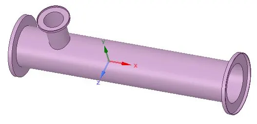
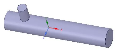
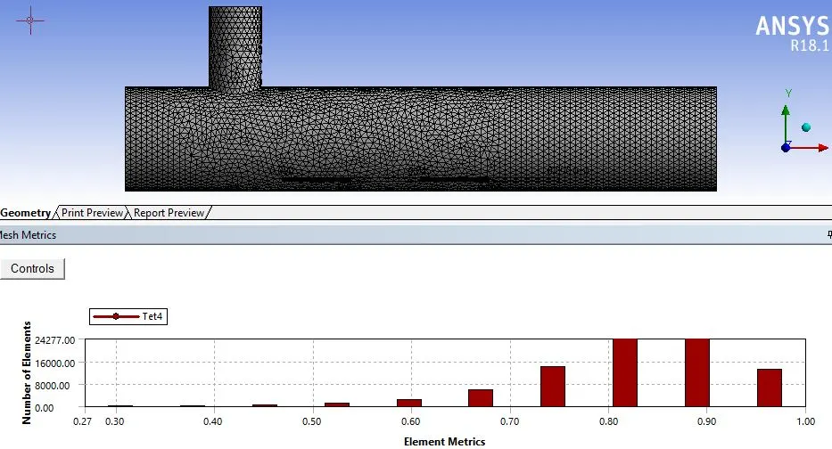
• Mesh – perform mesh and check mesh quality

• Setting up physics
  • General setting – steady state, pressure based solver
  • Model selection – Energy equation (on as heat transfer is involved), Turbulence model
  • Material selection – default material is air.
  • Boundary conditions – inlet velocity (hot) = 3m/s & temperature = 309.15 K, inlet velocity (cold) = based on momentum ratio & temperature = 292.15 K, outlet pressure = 0
  • Definitions – Area averaged – Temperature at outlet, Standard deviation – temperature at outlet
  • Initialization – Hybrid initialization at t=0 for setting up initial conditions
  • Calculation – enter no of iterations
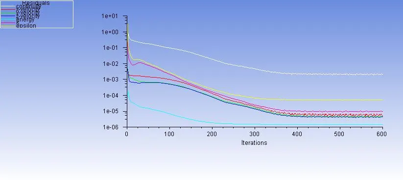
• Check for convergence based on the residual plots, temperature plots. When values remain constant or change is repetitive with respect to increasing iterations.
• Results – create a mid-plane along XY plane along the length of the tube. Plot temperature and velocity to see the results.
• Results -> Calculation – for the value of temperature at the outlet
  

Below is the flow of our study

• Turbulence model comparison
• Mesh independent study
• Baseline model study for 4 cases

Case 1 – V (h) = 3m/s, MR = 2, short pipe

Case 2 – V (h) = 3m/s, MR = 4, short pipe

Case 3 – V (h) = 3m/s, MR = 2, long pipe

Case 4 – V (h) = 3m/s, MR = 2, long pipe

Turbulence model comparison

• Here case 1 i.e. velocity at hot inlet = 3 m/s, velocity at cold inlet = 6 m/s for short pipe is explored. The case is simulation with K- ε and K-ω and results are reviewed. Based on that the model selection is done for the further study.
• The procedure followed for the simulation is same as above. The mesh size is baseline 2 mm.

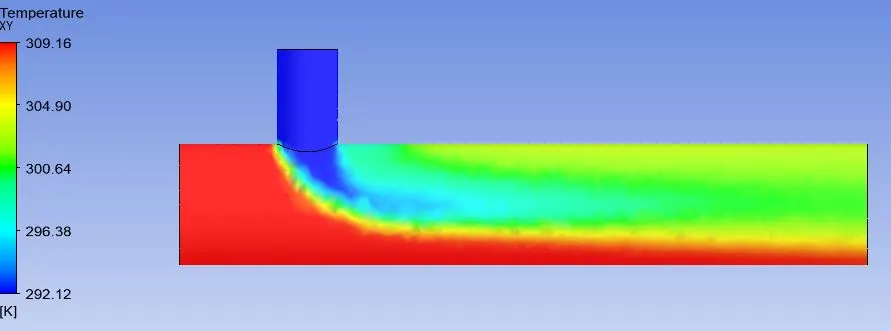
K- ε, standard wall function

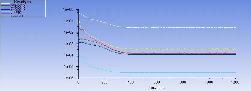
Solution Convergence – 400 to 450 iterations

Temperature contour

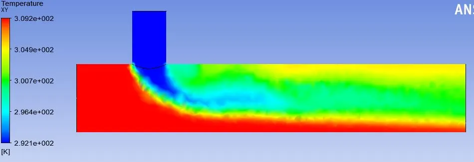
K- ω, standard wall function

Solution convergence – 300 iterations

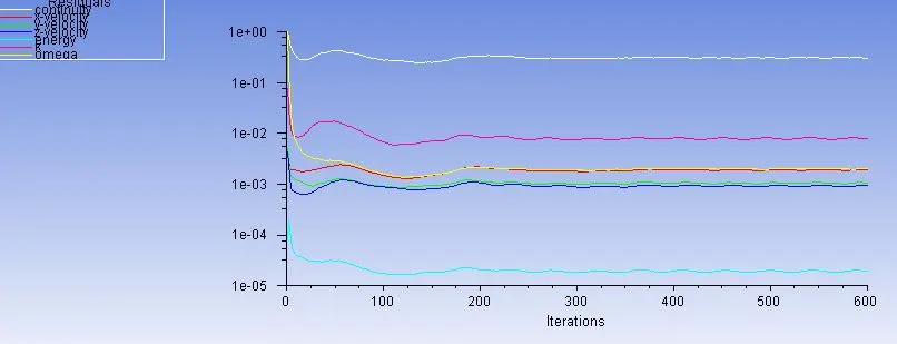
Temperature contour

Baseline Model
	K-E	K-W
Temperature (K)	303.408	303.609

From the above results we can see that the temperature profile in both the cases is almost similar. Also the outlet temperature is almost similar. As discussed earlier, both the method has its specific application as K- ε predicts well far from wall whereas K- ω predicts well near wall. This doesn’t have any considerable effect as we are not concerned with the wall interaction and thus either model can be used for our study. So we will proceed with K- ε, standard wall function for further study

Mesh Independent Study

• For this case 1 is taken. Velocity at hot inlet = 3 m/s & temperature = 309.15 K, velocity at cold inlet = 6 m/s & temperature = 292.15 K. K- ε, standard wall function
• Different mesh size of 2mm, 1mm, 0.75mm and 0.5mm are studied.

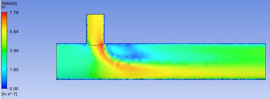
Mesh size = 2mm

Solution convergence – 400 to 450 iterations

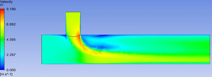
Temperature contour

Velocity contour

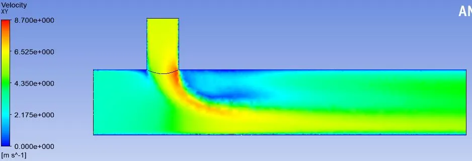
Mesh size = 1 mm

Solution convergence – 509 iterations

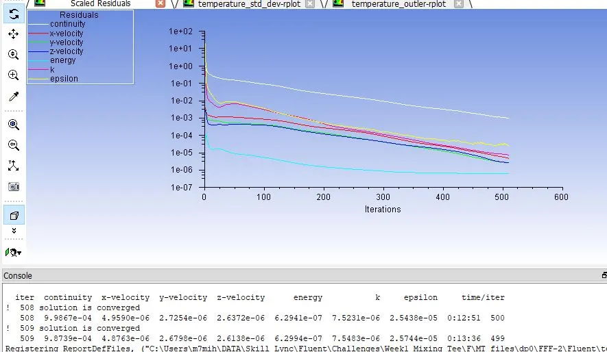
Temperature contour

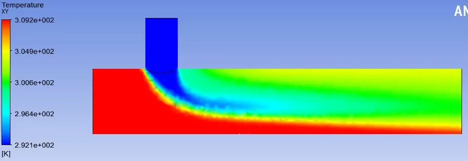
Velocity contour

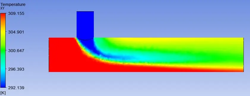
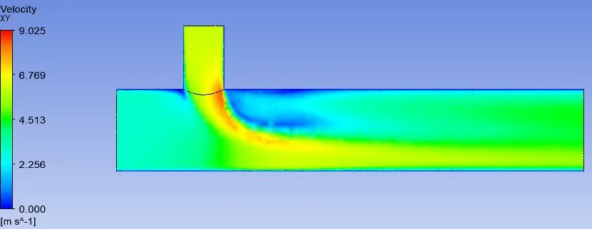
Mesh size = 0.75 mm

Solution convergence – 557 iterations

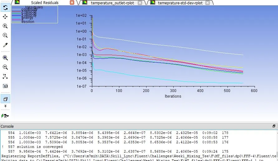
Temperature contour

Velocity contour

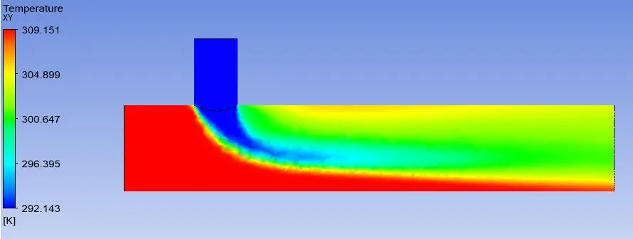
Mesh size = 0.5 mm

Solution convergence – 604 iterations

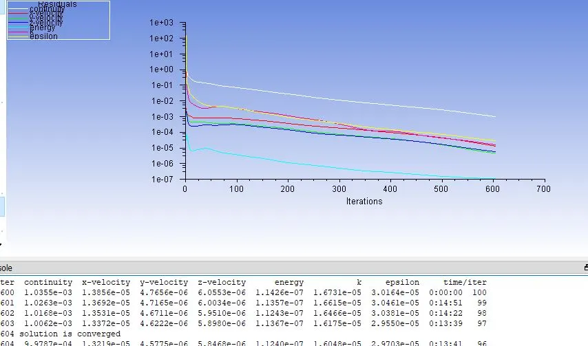
Temperature contour

Velocity contour

K-E Model
Mesh Size	2 mm	1mm	0.75 mm	0.5 mm
Temperature (K)	303.408	303.57	303.61	303.633

From the above table we can see that the solution becomes mesh independent after mesh size of 0.5 mm

Model Study

Although from above iterations, we found out that solution becomes mesh independent at mesh size of 0.5 mm, we will continue our study for the baseline mesh size of 2 mm as the difference in the final outlet temperature is minimal and save computation time. The problem will be solved using K- ε, standard wall function and standard mesh size of 2mm.

Short Mixing Tee

Case 1 – It is already discussed in detail in mesh independent study

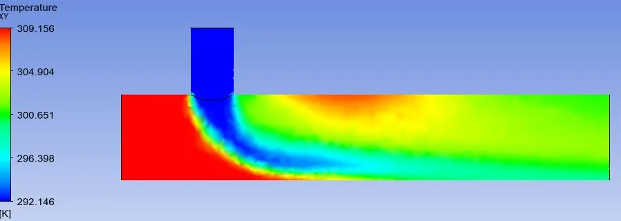
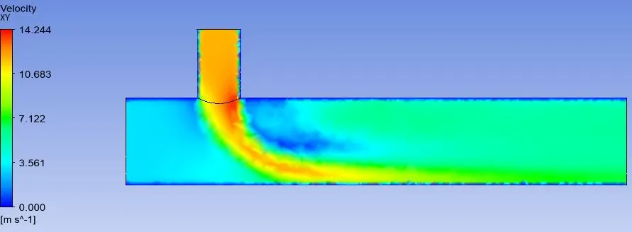
Case 2 – Velocity at hot inlet = 3 m/s & T = 309.15 K, Velocity at cold inlet = 12 m/s & T = 292.15 K, Momentum ratio = 4

Solution Convergence – 400 to 450 iterations

Temperature contour

Velocity contour

Long Mixing Tee

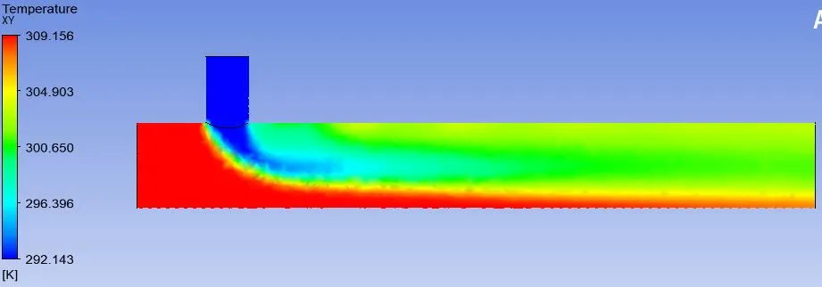
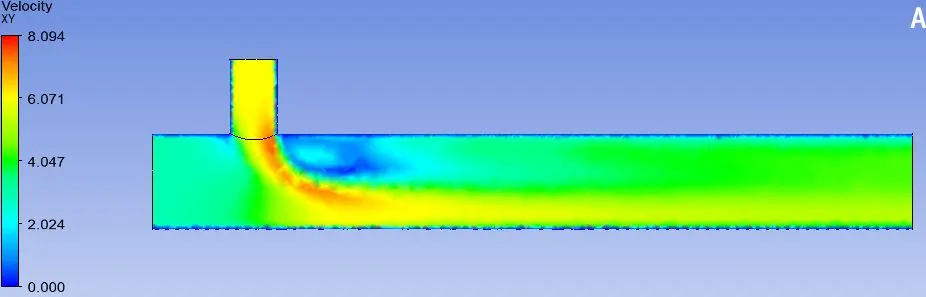
Case 3 – Velocity at hot inlet = 3 m/s & T = 309.15 K, Velocity at cold inlet = 6 m/s & T = 292.15 K, Momentum ratio = 2

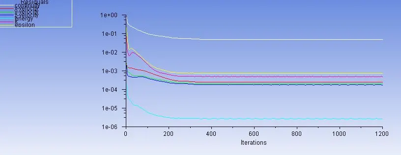
Solution Convergence – 350 iterations

Temperature contour

Velocity contour

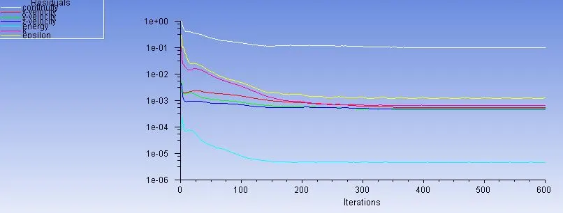
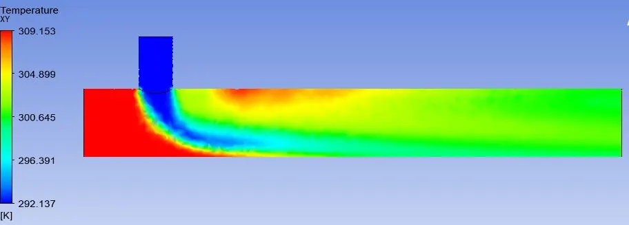
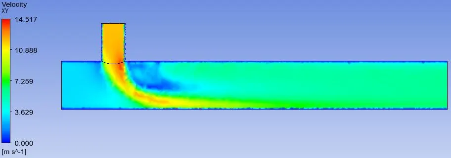
Case 4 – Velocity at hot inlet = 3 m/s & T = 309.15 K, Velocity at cold inlet = 12 m/s & T = 292.15 K, Momentum ratio = 4

Solution Convergence – 300 to 350 iterations

Temperature contour

Velocity contour

The temperature at outlet, mesh counts, node counts and convergence iterations can be summarized as follows.

Baseline mesh 2mm KE model
	Element Count	Node Count	Momentum Ratio	Convergence iterations	Temperature (K)
Short Mixing Tee	84854	17607	2	400-450	303.408
	84854	17607	4	400-450	300.706
Long Mixing Tee	117011	24165	2	350	303.519
	117011	24165	4	300-350	300.651

From the above table, we can say that there is not significant impact of length of mixing tee on the effectiveness. Instead the momentum ratio play an important role in efficiency. The main reason behind this when momentum ratio is 2 the cold fluid and hot fluid doesn’t mix as well as when momentum ratio is 4. So we can say that the effectiveness of the mixing tee is directly proportional to the difference in velocity of cold inlet and hot inlet

CONCLUSION

This study help us understand the basic steps involved in setting up a CFD problem and extracting the results. Also it gives an insight on how mixing of two fluid is affected.