Mid term project - Steady vs unsteady state analysis
AIM: To Compare the convergence rate [Number of iterations] of the steady state and transient [explicit and implicit] simulations and justify the numerics.
In the last Challenge [2D heat conduction], we have concluded that of all the given methods and approaches, the Successive Over-Relaxation method has been the most efficient. The fastest steady state simulation was confirmed by the Successive Over-Relaxation method and for the transient state simulation, it was the explicit SOR method.
TRANSIENT CASE:
In the transient case the program is solved by two methods,
- Explicit method
- Implicit method
The explicit method is solved directly since all the values are known.
In the implicit method all the values are Unknown, So the iterative techniques are used. Which are,
- Jacobi method
- Gauss seidal method
- SOR method
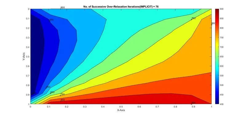
SUCCESSIVE OVER RELAXATION[STEADY-STATE]:
SUCCESSIVE OVER RELAXATION[UNSTEADY-STATE]:
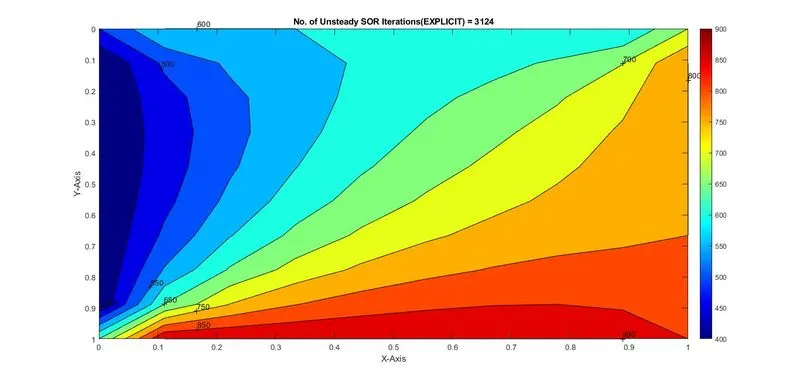
From the above stats, we can conclude that the Steady SOR method is the fastest of both the methods. But, it is also important to consider that the steady state does not include the Thermal Diffusivity and the time derivative terms which result in a steady and a fast solution. Similarily, the transient state SOR method involves mentioned earlier terms which result in higher simulation time and iterations when compared to the steady state SOR method.
In the case of transient simulations, the implicit approach is generally more stable than the explicit. It is so because when time steps are considered, explicit approaches are very sensitive to them and if a wrong time step is considered the solution may end up resulting in unstability. On the contrary, implicit solution approaches are less sensitive to time steps. This tells us that when a solution is solved implicitly, we may end up with higher simulation time and iterations which may be very expensive or wastage of valuable simulation time. In other words, we can also say that explicit solution approaches take less simulation time and iterations as the spatial nodes are solved seperately as a system of linear equations and the time integration here is similar to the convergence loop in the steady state simulation.
The Thermal Diffusivity (TD) also factors as an important consideration for our solvers. The right TD value leads to a more accurate solution. Considering we have the right value, other parameters like optuimum grid size and time steps also take priority for an accurate and fast solution. On the same note, we have also concluded in previous challenges that having a smaller time step will give is more precise and accurate results but may end up having larger simulation time. These are some of the factors and conditions which should be addressed when simulations of above nature are conducted. An exact range of these factors cannot be given as they change with the given problem and its specifications.