Combined Slip Tire Models - Brush Tire Model and Pacejka Tire Model
Problem Statement - 1:
Analyse the effect of slip angles (2 through 10 deg in increments of 2) on the Fx vs Fy relationship via the combined slip brush model for the slip ratio range of 0 to 1 (0 to 100%)
Deliverables:
Plot showing the effect of different slip angles on Fx vs Fy relationship
Data:
Solution:
Background Theory:
The elastic band model or brush model was proposed by Julian which initially explained the relationship between the longitudinal force and lonitudinal slip using the fore-aft deflection of brushes.
Julian's theory:
- Tire treads are considered to be elastic bands or brushes.
- The contact patch is rectangular.
- The pressure distribution in the contact patch is uniform.
- The contact patch is divided into adhesion region and sliding region.
The brush model consists of a row of elastic bristles that touches the road plane and can deflect in a direction parallel to the road surface. These bristles may be called tread elements. Their compliance represents the elasticity of the combination of carcass, belt and actual tread elements of the real tyre. As the tyre rolls, the first element that enters the contact zone is assumed to stand perpendicular with respect to the road surface. When the tyre rolls freely (that is without the action of a driving or braking torque) and without side slip, camber or turning, the wheel moves along a straight line parallel to the road and in the direction of the wheel plane. In that situation, the tread elements remain vertical and move from the leading edge to the trailing edge without developing a horizontal deflection and consequently without generating a fore and aft or side force. A possible presence of rolling resistance is disregarded. When the wheel speed vector V shows an angle with respect to the wheel plane, side slip occurs.
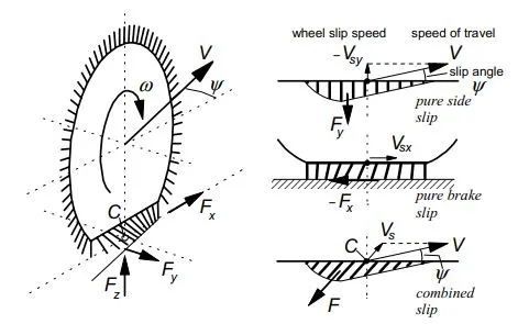
Combined Slip Brush Tire Model:
By employing the brush model we can evaluate forces in pure slip conditions i.e. longitudinal and lateral forces for corresponding slip ratios and slip angles. However in the real world driving phenomenon the combined cornering + braking/accelerating manoeuvre is executed quite often. Thus it is essential to evaluate this phenomenon in terms of resultant force generated as a result of the individual pure slip forces (longitudinal and lateral forces). Therefore the brush model which initially modeled the pure slip phenomenon is developed to represent the combined slip phenomenon. Hence, the combined slip model deals with the combined tractive and cornering forces. The peak value of the resultant combined force is governed by a curve of radius `mu*F_(z)`
where
`mu -` Friction coefficent
`F_(z) -` Normal load acting on the tire
This curve is termed as the Friction circe or Friction ellipse which is indicative of the capability of the tire in the combined cornering + braking/ acceleration manoeuvre.
This curve is generated using Matlab and depicts only the first quadrant and the effect of specified slip angles on the tire capability for the cornering + braking manoeuvre.
Matlab Script:
%Combined_slip_brush_tyre_model
%Combined_Braking/Cornering_case

%%
clear all;
clc;

%%
%Input parameters
Fz   = 5000;
mu   = 0.85;
lt   = 0.2;
kt   = 3.5*10^6;
ky   = 2.5*10^6;

%%
%Compute stiffnesss coefficients
C_x = (kt*lt^2)/2;
C_alpha = (ky*lt^2)/2;

%%
for k = 2:2:10;
alpha = k*(pi/180);

for g = 1:201   %Sweep of slip angles from 2 to 10 deg with increment od 2 deg
    Sb   = (g-1)*0.005;
    temp = ((C_x*Sb)^2+(C_alpha*tan(alpha))^2)^0.5;
    lc   = mu*Fz*(1-Sb)*lt/(2*temp);

    if lc >= lt
        Fx(g) = C_x*Sb/(1-Sb);
        Fy(g) = C_alpha*tan(alpha)/(1-Sb);
    else
        Fx(g) = mu*Fz*C_x*Sb/temp*(1-mu*Fz*(1-Sb)/(4*temp));
        Fy(g) = mu*Fz*C_alpha*tan(alpha)/temp*(1-mu*Fz*(1-Sb)/(4*temp));
    end
end

%Plot

figure(1)
plot(Fx,Fy,'linewidth',2);
hold on;
grid on;
set (gca,'fontsize',9);
title('Combined Slip Lateral Force vs. Longitudinal Force');
xlabel('Longitudinal Force (N)');
ylabel('Lateral Force (N)');
legend ('alpha = 2 deg ','alpha = 4 deg ','alpha = 6 deg ','alpha = 8 deg ','alpha = 10 deg ');
end
Script link:
https://drive.google.com/file/d/1hSxhS1rduuu_vrC2OCw5FYsRhzWcAn9j/view?usp=sharing
Plot:
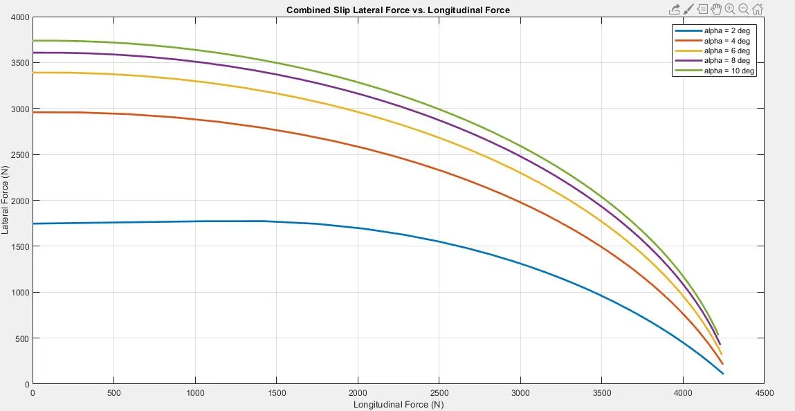
Inference:
Here we can see that the lateral force is proportional to the tire slip angles. Also as the slip angles go on increasing the difference in the consecutive peak values of the lateral force goes on decreasing (can be seen on the Y-axis at zero longitudinal force) which is indicative of the tire achieving the saturation point and the contact patch moving to the sliding region.
Now for a constant slip angle it can be concluded that as the longitudinal force goes on increasing the lateral component of the resultant force decreases resulting in a net understeer or oversteer effect on the vehicle. Also as we increase the longitudinal force the deviation in the lateral force for consecutive slip angle decreases and saturates to zero.
Problem Statement - 2:
- Analyse the effect of different slip ratios on longitudinal and lateral force vs. slip angle relationship. The slip ratios range is from 0% to 9% with increment of 3 and the sweep of the slip angle is from 0 deg to 20 deg.
- Analyse the effect of different slip angles on longitudinal and lateral force vs. slip ratio relationship. The slip angle range is from 0deg to 6deg with increment of 2deg and the sweep of the slip ratio is from 0% to 60%.
Deliverables:
Case 1:
-
Plot showing the effect of different slip ratios on lateral force vs slip angle relationship.
-
Plot showing the effect of different slip ratios on longitudinal force vs slip angle relationship.
Case 2:
-
Plot showing the effect of different slip angles on llateral force vs slip ratio relationship.
-
Plot showing the effect of different slip angles on longitudinal force vs slip ratio relationship.
Data:
| Lateral factors | |
| Peak Slip angle | 4 deg |
| By (Stiffness factor) | 0.27 |
| Cy (Shape factor) | 1.2 |
| Dy (Peak factor) | 2900 |
| Ey (Curvature factor) | -1.6 |
| Shy (Horizontal shift) | 0 |
| Svy (Vertical shift) | 0 |
| Longitudinal factors | |
| Peak slip ratio | 9 % |
| Bx (Stiffness factor) | 25 |
| Cx (Shape factor) | 1.25 |
| Dx (Peak factor) | 3200 |
| Ex (Curvature factor) | -0.4 |
| Shx (Horizontal shift) | 0 |
| Svx (Vertical shift) | 0 |
Solution:
Background theory:
The Pacejka tire model was developed by Hans. B Pacejka of the Delft University of Technology. It is an empirical tire model also known as the magic formula and is widely used for simulation purposes.
The model provides a set of mathematical expressions from which the forces and moment acting on the tire can be calculated at pure slip and combined slip conditions. The model aims at an accurate description of measured tire behaviour obtained from the physical tests by providing a near ideal curve fit with the measured data points. The coefficients of the mathematical expression represent the tire characteristics. By selecting proper values, the characteristics for either longitudinal force, lateral force and aligning moment can be obtained.
The generalised Pacejka tire model expression:
`y(x)=D*sin[C*tan^(−1){Bx−E(Bx−tan^(−1)(Bx))}],`
`Y(x) = y(x) + Sv`
`x = X + Sh`
where,
`y(x) −` Output - Longitudinal force, Lateral force or Aligning moment
`x −` Input - Slip angle or Slip ratio
`D −` Peak factor
`C −` Shape factor
`B −` Stiffness factor
`E −` Curvature factor
`Sh −` Horizontal shift
Vertical shift
The vertical and horizontal offsets take into account the camber thrust, conicity, ply steer or rolling resistance.
For combined slip condition:
In the combined slip condition (cornering + acceleration or cornering + braking) both the longitudinal and lateral forces are in play. In pure slip condition longitudinal force is a function of slip ratio and the lateral force is the function of slip angle. On this fundamental tire behaviour the combined slip phenomenon is analysed with the Pacejka tire model.
Given are the following parameters:
`S_x −`Slip ratio
`S_(xp) -`Peak slip ratio
`α −`Slip angle
`α_p −`Peak slip angle
From the above parameters the normalized slip parameters are determined:
`S_(x)^ast = (S_x/S_(xp))`
`α^∗ = (α/α_p)`
Further the resultant slip of the tire is determined:
`S^∗ = sqrt((S_x^ast)^2+(α^∗)^2)`
The modified slip ratio and slip angle is determined:
`S_(xm) = S^∗*S_(xp)`
`α_m = S^∗*α_p`
Now the longitudinal force and lateral force is computed:
`F_x = F_(x0)*(S_(x)^ast/S^∗)`
`F_y = F_(y0)*(α^∗/S^∗)`
where,
`F_(x0) −` Longitudinal force calculated using the modified slip ratio using the Pacejka formula
`F_(y0) -`Lateral force calculated using the modified slip angle using the Pacejka formula
Considering the above formulations, deliverables are achieved from matlab script explained as follows:
For Case 1:
-
Plot showing the effect of different slip ratios on lateral force vs slip angle relationship.
-
Plot showing the effect of different slip ratios on longitudinal force vs slip angle relationship.
Matlab Script Explanation:
1. Clearing the command window and the workspace before code execution along with initialising and assigning values to the input variables stated in the problem statement for peak slip ratio and slip angle respectively.
%1_Effect of slip ratios on lateral force vs slip angle relationship
%2_Effect of slip ratios on longitudinal force vs slip angle relationship

%%
clear all;
clc;

%%
%Input Parameters
Sx_p    = 0.09;   %Peak slip is 9%
alpha_p = 4;      %Peak slip angle is 4 deg
2. Initialising and assigning values to the input variables of the Pacejka coefficients further used in the magic formula for formulating both lateral and lonitudinal forces.
%%
%Pacjecka Coefficients

%Lateral Force
By  = 0.27;
Cy  = 1.2;
Dy  = 2900;
Ey  = -1.6;
Shy = 0;
Svy = 0;

%Longitudinal Force
Bx  = 25;
Cx  = 1.15;
Dx  = 3200;
Ex  = -0.4;
Shx = 0;
Svx = 0;
3. Initialising the for loop calculating the lateral and logitudinal forces for a specific slip ratio (0%, 3%, 6% and 9%) and for a sweep of slip angles (0 deg to 20 deg). Generates slip ratios 0%, 3%, 6% and 9%.
%Iterate through four slip ratios
for g = 1:4
    Sx = (g-1)*0.03;
4. Initialising nested for loop generating the sweep of slip angle (0 deg to 20 deg).
%Generating a sweep of slip angles from 0 deg to 20 deg
    for h = 1:21
        slip_angle(h) = (h-1)+0.0000001;
        alpha = slip_angle(h);
5. Calculating the normalised slip parameters and corresponding lateral and longitudinal forces for the specified slip ratios (0%, 3%, 6% and 9%) and the slip angle sweep (0 deg to 20 deg).
a. Calculating normalised slip factors.
%Normalized slip factors
Sx_star    = Sx/Sx_p;
alpha_star = alpha/alpha_p;
b. Calculating resultant slip and modified slip factors.
%Resultant slip
S_star = ((Sx_star)^2 + (alpha_star)^2)^0.5;

%Modified slip factors
Sx_mod    = S_star*Sx_p;
alpha_mod = S_star*alpha_p;
c. Calculating lateral and longitudinal forces using the above calculated normalised slip parameters (slip and slip angles) in magic formula with the end of for loops.
%Lateral force calculation
alpha_final = alpha_mod + Shy;
fy(g,h)     = (alpha_star/S_star)*Dy*sin(Cy*atan(By*alpha_final-Ey*(By*alpha_final-atan(By*alpha_final))));
Fy(g,h)     = fy(g,h) + Svy;

%Longitudinal force calculation
Sx_final    = Sx_mod + Shx;
fx(g,h)     = (Sx_star/S_star)*Dx*sin(Cx*atan(Bx*Sx_final-Ex*(Bx*Sx_final-atan(Bx*Sx_final))));
Fx(g,h)     = fx(g,h) + Svx;
    end
end
6. Generating plot for the specified range of slip ratios of Lateral force vs. slip angle and Longitudinal force vs. slip angle.
Lateral force vs. Slip angle
%Plot
subplot(2,1,1);
plot(slip_angle,Fy,'linewidth',3);
set(gca,'fontsize',9);
xlabel('Slip angle (deg)');
ylabel('Fy (N)');
legend('skid = 0','skid = 0.03','skid = 0.06','skid = 0.09');
title('Lateral Force vs. Slip Angle','fontsize',9);
Longitudinal force vs. Slip angle
subplot(2,1,2);
plot(slip_angle,Fx,'linewidth',3);
set(gca,'fontsize',9);
xlabel('Slip angle (deg)');
ylabel('Fx (N)');
legend('skid = 0','skid = 0.03','skid = 0.06','skid = 0.09');
title('Longitudinal Force vs. Slip Angle','fontsize',9);
Plots:
Figure 1a: Lateral Force vs. Slip angle
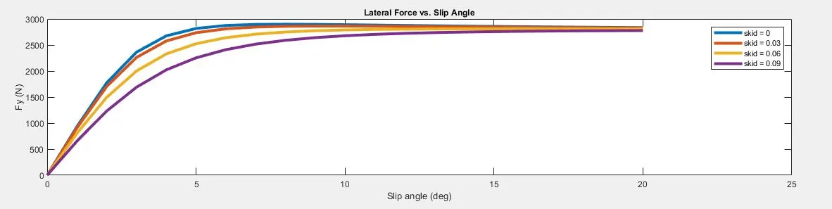
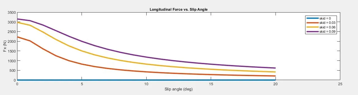
Figure 1b: Longitudinal Force vs. Slip angle
Inference:
Figure 1a:
The plot depicts an overall non linear trend of the lateral force vs. slip angle plot for a combined slip phenomenon. This is indicative of the adhesion region in the contact patch (initial linear trend), the partial sliding region (non linear transition between approx 2 deg to 5 deg) and total sliding region (beyond 5 deg). Also as the slip ratio increases the peak lateral force goes on decreasing which is indicative of larger contribution of the longitudinal force in the combined slip phenomenon. Also, lateral force increases with increase in slip angle but at high slip angles due to tire load sensitivity the force saturates for all slip ratio values.
Figure 1b:
At zero slip angle the longitudinal force is maximum for a particular value slip ratio. As the slip angle progressively increases the lateral force increases reducing the contribution of the longitudinal force. Also the initial difference between the succesive longitudinal forces corresponding to the slip ratio reduces at high slip angles depictin the major contribution of the lateral force.
For Case 2:
-
Plot showing the effect of different slip angles on lateral force vs slip ratio relationship.
-
Plot showing the effect of different slip angles on longitudinal force vs slip ratio relationship.
Matlab Script Explanation:
1. Clearing the command window and the workspace before code execution along with initialising and assigning values to the input variables stated in the problem statement for peak slip ratio and slip angle respectively.
%1_Effect of slip ratios on lateral force vs slip angle relationship
%2_Effect of slip ratios on longitudinal force vs slip angle relationship

%%
clear all;
clc;

%%
%Input Parameters
Sx_p    = 0.09;   %Peak slip is 9%
alpha_p = 4;      %Peak slip angle is 4 deg
2. Initialising and assigning values to the input variables of the Pacejka coefficients further used in the magic formula for formulating both lateral and lonitudinal forces.
%%
%Pacjecka Coefficients

%Lateral Force
By  = 0.27;
Cy  = 1.2;
Dy  = 2900;
Ey  = -1.6;
Shy = 0;
Svy = 0;

%Longitudinal Force
Bx  = 25;
Cx  = 1.15;
Dx  = 3200;
Ex  = -0.4;
Shx = 0;
Svx = 0;
3. Initialising the for loop calculating the lateral and logitudinal forces for a specific slip angles (0 deg, 2 deg, 4 deg and 6 deg) and for a sweep of slip ratios (0% to 60%). Generates slip angles 0 deg, 2 deg, 4 deg, 6 deg.
%Iterate through four slip angles
for g = 1:4
    slip_angle(g) = (g-1)*2;
    alpha = slip_angle(g);
4. Initialising nested for loop generating the sweep of slip ratio (0% to 60%).
%Generating the sweep of slip ratios from 0% to 60%
    for h = 1:61
        Sx(h) = (h-1)*0.01;
5. Calculating the normalised slip parameters and corresponding lateral and longitudinal forces for the specified slip angles (0 deg, 2 deg, 4 deg and 6 deg) and the slip ratio sweep (0% to 60%).
a. Calculating normalised slip factors.
%Normalized slip factors
Sx_star    = Sx(h)/Sx_p;
alpha_star = alpha/alpha_p;
b. Calculating resultant slip and modified slip factors.
%Resultant slip
S_star = ((Sx_star)^2 + (alpha_star)^2)^0.5;

%Modified slip factors
Sx_mod    = S_star*Sx_p;
alpha_mod = S_star*alpha_p;
c. Calculating lateral and longitudinal forces using the above calculated normalised slip parameters (slip and slip angles) in the magic formula with the end of for loops.
%Lateral force calculation
alpha_final = alpha_mod + Shy;
fy(g,h)     = (alpha_star/S_star)*Dy*sin(Cy*atan(By*alpha_final-Ey*(By*alpha_final-atan(By*alpha_final))));
Fy(g,h)     = fy(g,h) + Svy;

%Longitudinal force calculation
Sx_final    = Sx_mod + Shx;
fx(g,h)     = (Sx_star/S_star)*Dx*sin(Cx*atan(Bx*Sx_final-Ex*(Bx*Sx_final-atan(Bx*Sx_final))));
Fx(g,h)     = fx(g,h) + Svx;
    end
end
6. Generating plot for the specified range of slip angles of Lateral force vs. slip ratio and Longitudinal force vs. slip ratio.
Lateral force vs. Slip ratio
%Plot
subplot(2,1,1);
plot(Sx,Fy,'linewidth',3);
set(gca,'fontsize',9);
xlabel('Slip ratio');
ylabel('Fy (N)');
legend('slip angle = 0deg','slip angle = 2deg','slip angle = 4deg','slip angle = 6deg');
title('Lateral Force vs. Slip Angle','fontsize',9);
Longitudinal force vs. Slip ratio
subplot(2,1,2);
plot(Sx,Fx,'linewidth',3);
set(gca,'fontsize',9);
xlabel('Slip ratio');
ylabel('Fx (N)');
legend('slip angle = 0deg','slip angle = 2deg','slip angle = 4deg','slip angle = 6deg');
title('Longitudinal Force vs. Slip Angle','fontsize',9);
Plots:
Figure 2a: Lateral Force vs. Slip ratio
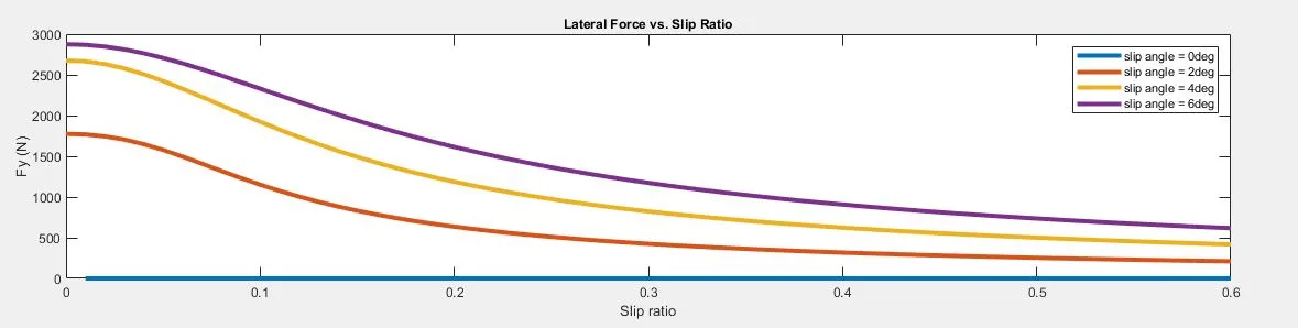
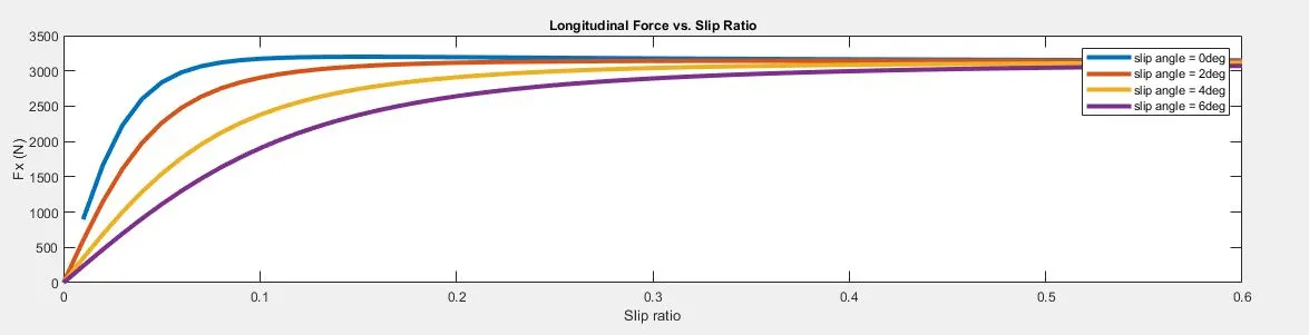
Figure 2b: Longitudinal Force vs. Slip ratio
Inference:
Figure 2a:
It is evident from the plot that the lateral force is maximum for a corresponding slip angle at 0 % slip with a significant difference in the force values for consecutve slip angle in the lower range (2 deh - 4 deg) and a relatively reduced difference between the values corresponding to slip angles in the higher range (4 deg - 6 deg) indicative of the saturation limit of the tire. Also as the slip ratio increases the lateral force decreases with a reduced difference in the consecutive force values corresponding to the specified slip angles. This is indicative of the saturation of the lateral force.
Figure 2b:
The plot depicts that at high slip angle the peak longitudinal force reduces as the slip ratio increases. This reduction saturates at high slip ratios operating the tire in the sliding region. Also the logitudinal force increases linearly for initial slip ratio values and saturates at high slip ratio values for a particular slip angle.