Gate Valve Parametric Study
OBJECTIVE
- Setup gate disc lift as an input parameter and mass flow rate at the outlet as an output parameter
- Perform the CFD simulation for gate disc lift varying from 10% to 80%
- Extract mass flow rate at the outlet, flow coefficient, and flow factor.
- Discuss the results.
THEORY
Gate Valve
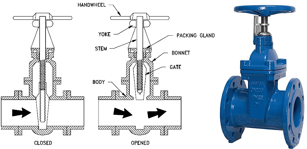
A gate valve, also known as a sluice valve, is a valve that opens by lifting a barrier (gate) out of the path of the fluid. Gate valves require very little space along the pipe axis and hardly restrict the flow of fluid when the gate is fully opened.
A gate valve's main components are body, seat, gate, stem, bonnet, and actuator. The primary operation mechanism is straightforward. Turning the handwheel rotates the stem, which moves the gate up or down via the threads. They require more than one 360° turn to fully open/close the valve. Lifting the gate from the path of the flow, the valve opens. Lowering the gate to its closed position seals the bore resulting in a full closure of the valve. For a gate valve, the relationship between the gate's vertical travel and the flow rate is nonlinear, with the highest changes occurring near shutoff.
Parametric Study in Fluent
Often while performing a CFD analysis, different simulations are run just by changing an input parameter. So instead of setting up the simulation case each time, the Parameters option can be utilized to setup up the case only once and use the same setup to run the case multiple times without manually changing the input parameters.
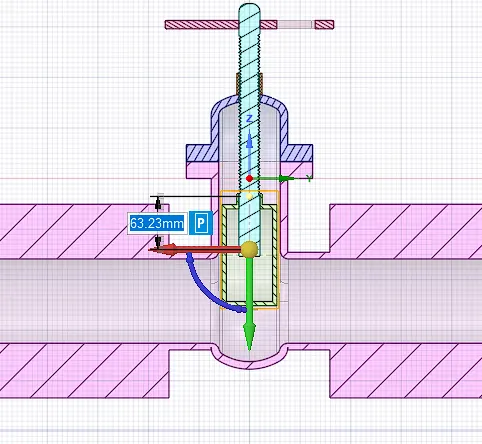
This can be activated by pressing the P option in the geometry phase. Also in order to create the same output for each input, we can create the output parameters option available.
Flow Coefficient and Flow factor
- The flow coefficient of a device is a relative measure of its efficiency at allowing fluid flow. It describes the relationship between the pressure drop across an orifice valve or other assembly and the corresponding flow rate.
`Cv = Qsqrt[(SG)/(ΔP )`, Q = flow rate in gallons per min, SG = specific gravity of fluid, ΔP = pressure drop across the valve in psi
- Flow factor is the metric equivalent of flow coefficient in SI unit and is denoted by Kv
`Kv = 0.862 Cv`
PROCEDURE
Following steps are followed in setting up the case.
Step 1 - Geometry setup
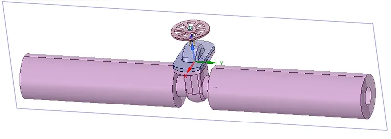
- Import the gate valve geometry in SpaceClaim
- Use the pull option to pull the surface to replicate the pipe domains.
- Move the disc up and create a parameter group.
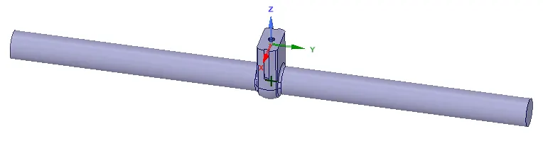
- Prepare -> Volume extract. Suppress the original geometry for physics.
Step 2 - Meshing
- Create a fine mesh and check the mesh quality

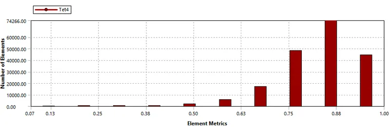
- Assign named selection for inlet and outlet of the flow
Step 3 - Setting up the Physics
- Solver - Pressure based steady-state solver. gravity = 9.81 m/s2
- Model - k-Epsilon -> Realizable -> Scalable wall function, since the flow is turbulent
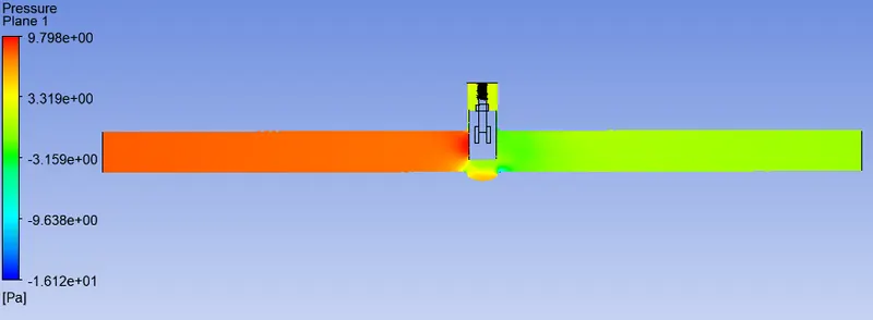
- Boundary condition -> inlet -> pressure inlet -> edit -> pressure = 10 pa, Outlet -> pressure = 0 Pa
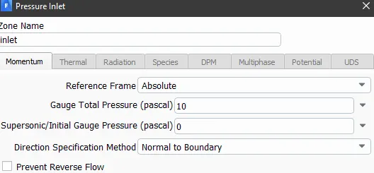
- Monitor point -> Definitions -> Flux report -> mass flow rate -> outlet -> create output parametes
- Create contours -> pressure and velocity
Step 4 - Inititalization
- Standard Initialization -> Compute from inlet -> initialize
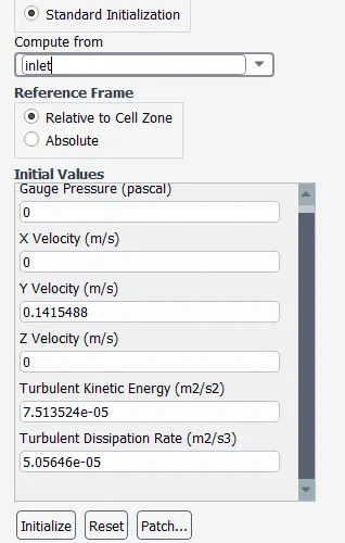
Step 5 - Run the simulation
Step 6 - Create design point
- Exit the Fluent and create design points using parameters tab in Workbench.
- enter gate disc opening distance and select retain data. Total 8 cases with opening 10mm, 20mm, 30mm, 40mm, 50mm, 60mm, 70mm, and 80mm were considered.
- Solve all
Step 7 - Results
RESULTS
Below image shows the design points used in conducting the parametric study. It shows the disc opening and mass flow rate.
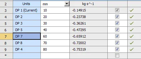
Each case is listed below
Case 1 - 10 mm gate disc opening
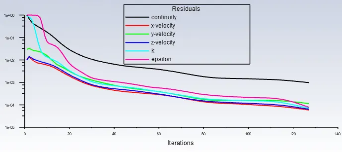
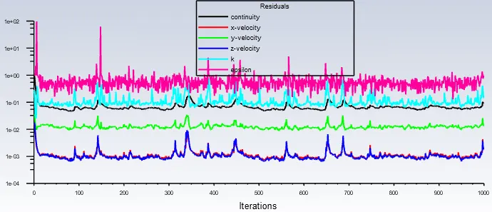
- Residual
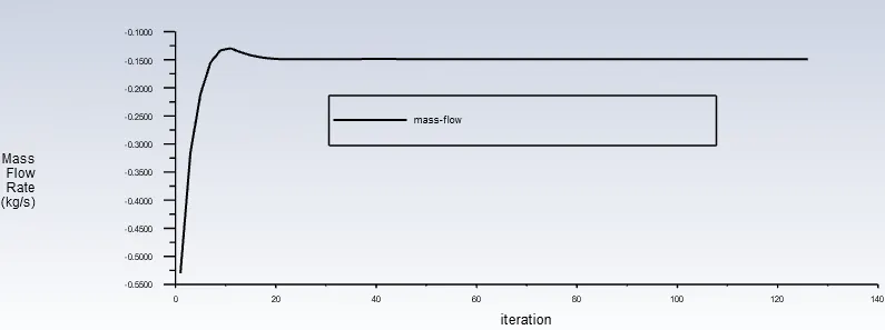
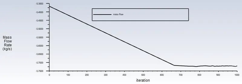
- Mass Flow Rate
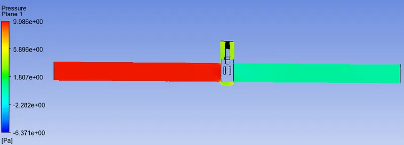
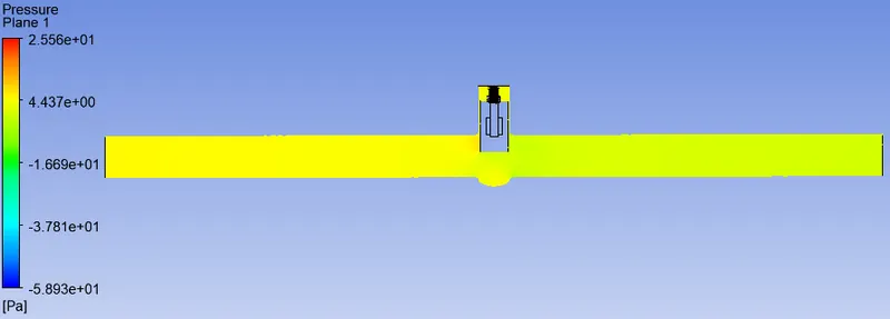
- Pressure Contours
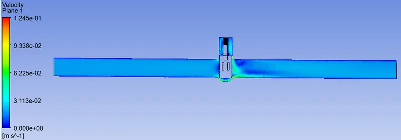
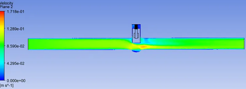
- Velocity Contours
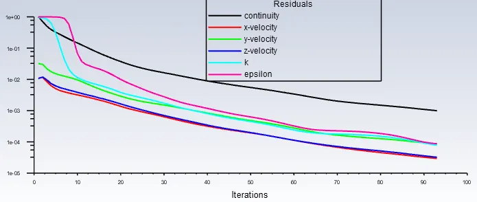
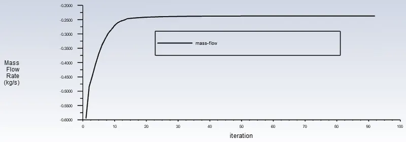
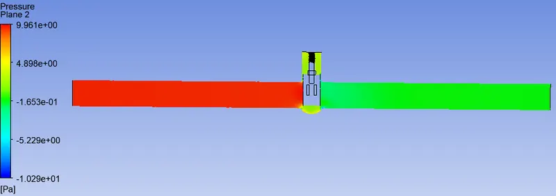
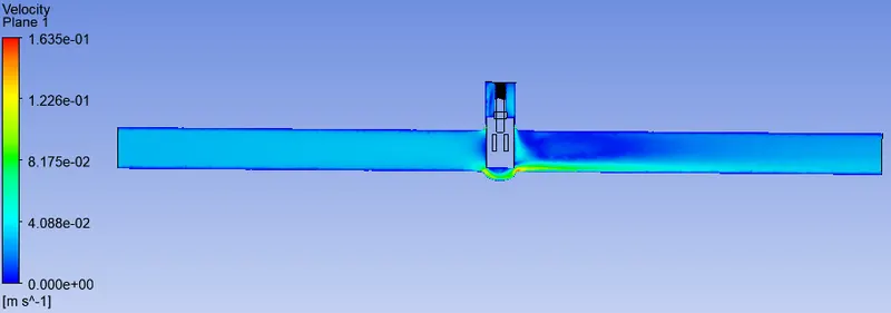
Case 2 - 20 mm gate disc opening
- Residual
- Mass Flow Rate
- Pressure Contours
- Velocity Contours
Case 3 - 30 mm gate disc opening
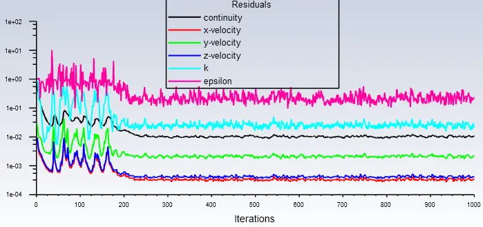
- Residual
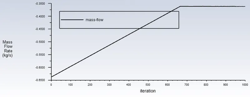
- Mass Flow Rate
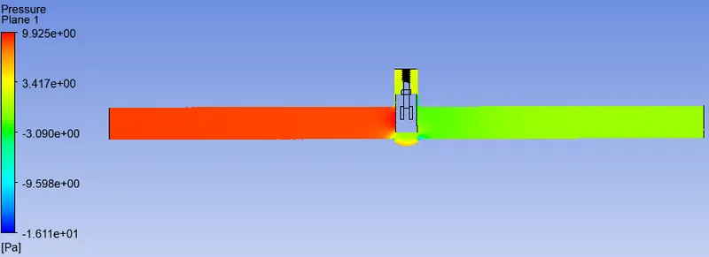
- Pressure Contours
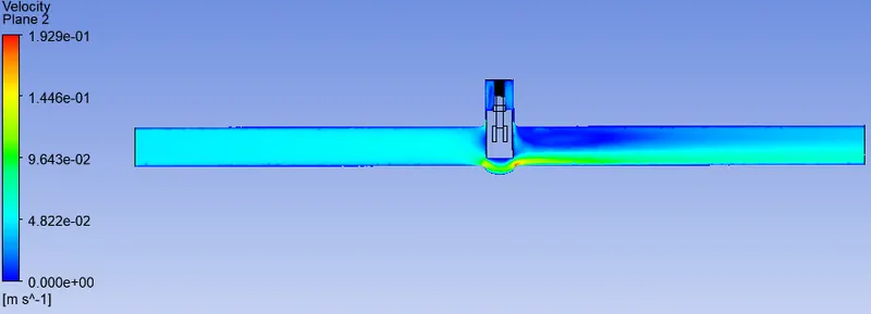
- Velocity Contours
Case 4 - 40 mm gate disc opening
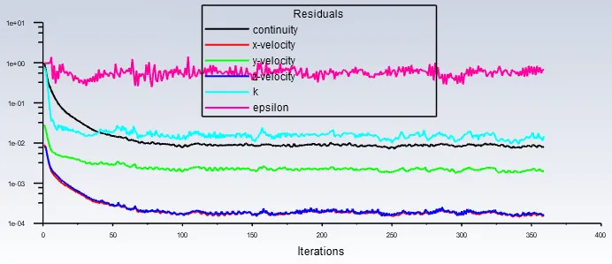
- Residual
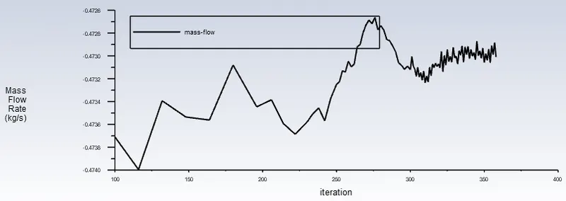
- Mass Flow Rate
- Pressure Contours
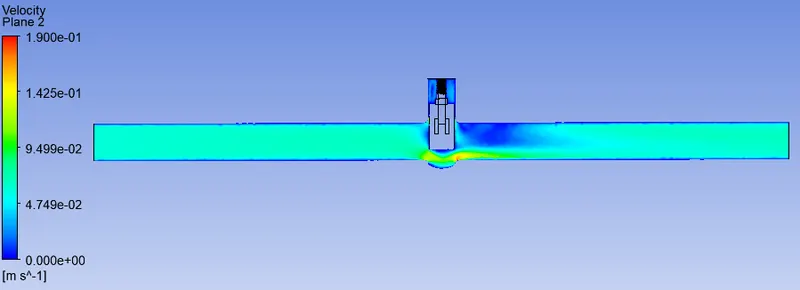
- Velocity Contours
Case 6 - 60 mm gate disc opening
- Residual
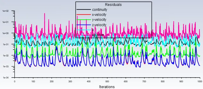
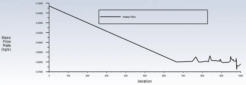
- Mass Flow Rate
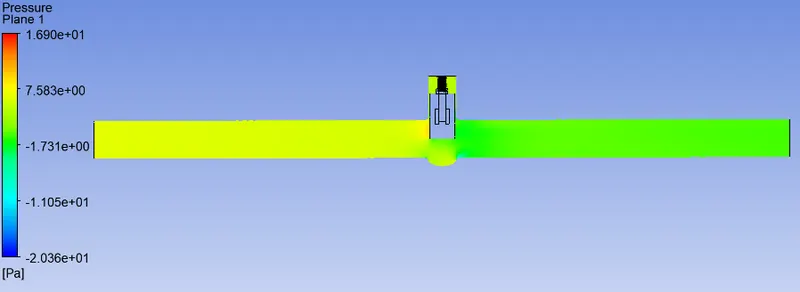
- Pressure Contours
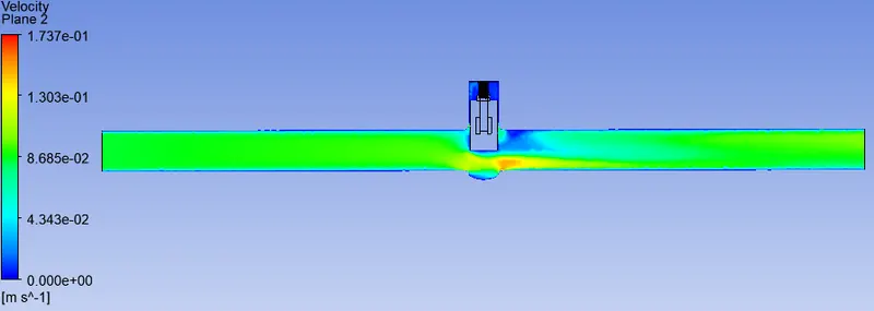
- Velocity Contours
Case 7 - 70 mm gate disc opening
- Residual
- Mass Flow Rate
- Pressure Contours
- Velocity Contours
Case 8 - 80 mm gate disc opening
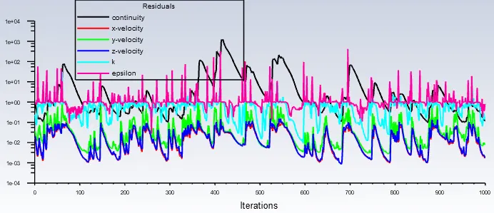
- Residual
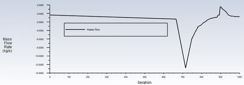
- Mass Flow Rate
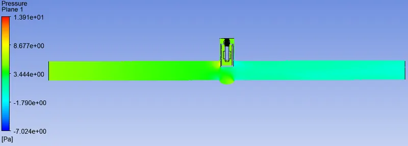
- Pressure Contours
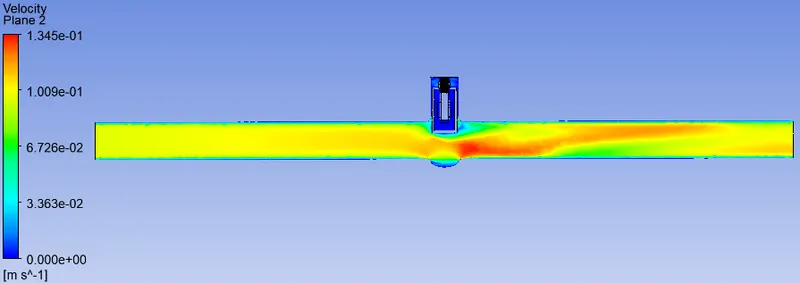
- Velocity Contours
Now in our case, the fluid is taken as water and thus the specific gravity of the fluid is 1. So for the calculation of flow coefficient and flow factor
`Cv = Qsqrt[(SG)/(ΔP )`
For case 1, Cv = (3.1975) sqrt (1/0.00145) = 83.9705.
`Kv = 0.862 Cv` = 0.862 *83.9705 = 72.23825
Similarly the flow coefficient for each case was extracted
| Case | Lift (mm) | Mass Flow Rate (kg/s) | Mass Flow Rate (gallon/min) | Pressure (Pa) | Pressure (psi) | Flow Coefficient | Flow Factor |
| 1 | 10 | -0.14915 | -3.1975 | 10 | 0.00145 | 83.9705 | 72.23825 |
| 2 | 20 | -0.23738 | -5.0891 | 10 | 0.00145 | 133.646 | 115.203 |
| 3 | 30 | -0.36261 | -7.7739 | 10 | 0.00145 | 204.153 | 175.98 |
| 4 | 40 | -0.47295 | -10.1394 | 10 | 0.00145 | 266.274 | 229.528 |
| 6 | 60 | -0.65912 | -14.1307 | 10 | 0.00145 | 371.09 | 319.88 |
| 7 | 70 | -0.72002 | -15.4363 | 10 | 0.00145 | 405.377 | 349.435 |
| 8 | 80 | -0.75319 | -16.1478 | 10 | 0.00145 | 424.062 | 365.341 |
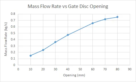
Mass Flow Rate vs Gate Disc Opening
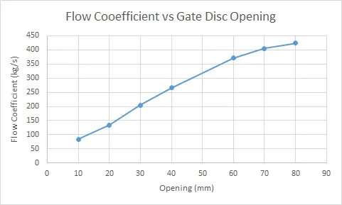
Flow Coefficient vs Gate Disc Opening
CONCLUSION
The above challenge helped us understand the working procedure of conducting a parametric study. Also based on the results discussed in previous section following points can be concluded
- Based on the above discuss results, we can see that mass flow rate and flow coefficient increases with the increase in gate disc opening.
- The velocity of the flow also increase with the increase in disc opening.
- The increase in mass flow is non linear and thus cannot be predicted based on amount of gate disc lifted.
Important point to consider while performing the parametric study is the no of iterations and convergence criteria. Since the solver solves the design points based on the 1st case setup, the results maybe affected as the solution may stop before reaching the convergence as no of iterations runs out or if the convergence criteria is met but our desired output may not have converged. So a check must be performed.