Flow over bicycle

AIM: To write a Python program to calculate drag force against a cyclist.

OBJECTIVES:

• Write a program to plot Velocity vs Drag force.
• Write a program to plot Drag Co-efficient vs Drag force.

CODE:

import math
import matplotlib.pyplot as plt


#Initialisation of parameters
n = 15
rho = 1.225  # kg/m^3
frontal_area = 0.51  # m^2
velocity = []  # m/sec
Drag_Force = [] #kg-m/s^2
C_d = [1.1, 0.88, 0.5, 0.12]  # Different Cd based on different shapes of frontal area
temp=[]

#filling velocity vector
for i in range(1, n + 1):
    velocity.append(i)


Drag_Force_for_vel1=[] #to store drag force for vel=1m/s

#plot 1
for cd in C_d:

    for v in range(0,n):
        temp = (1/2)*(rho)*(frontal_area)*(pow(velocity[v],2))*cd
        Drag_Force.append(temp)
        #print(Drag_Force)
    Drag_Force_for_vel1.append(Drag_Force[0])
    plt.plot(velocity, Drag_Force)
    plt.xlabel('Velocity')
    plt.ylabel('Drag Force')
    temp=[cd]
    plt.legend(temp)
    plt.show()
    Drag_Force=[]


#plot 2
#print(Drag_Force_for_vel1)
plt.plot(C_d, Drag_Force_for_vel1)  
plt.xlabel('C_d')
plt.ylabel('Drag_Force_for_vel=1m/sec')
plt.show() 

OUTPUTS:

1)Plot 1:

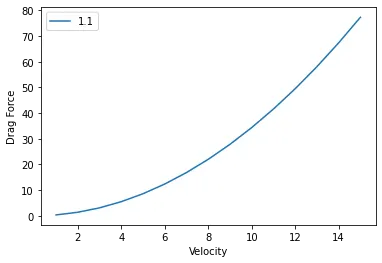
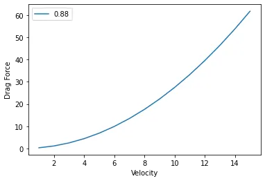
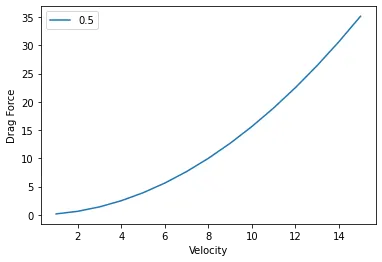
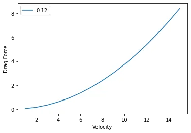
Thus, from the above plots, we can observe the parabolic relation between drag force and velocity and how drag force increases as drag coeff. increases for different velocities.

2)Plot 2:

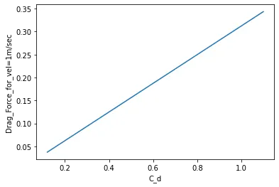
NOTE:For plot 2, I have used only one value of velocity (v=1m/sec).

EXPLANATION:

1)First we initialised variables with given parameters.

2)To create the velocity matrix, we used a for loop and loopes it fifteen times for storing the velocity values one by one using the append() command.

3)Under #plot 1, we will be calculating drag force and also simultaneously plot for the corresponding C_d value. Thus, for each C_d value, we have calculated the drag force for different velocities. Thus, we can see two for loops.

4)Finally, to plot both the curves, we use plt.plot() command.