Flow over a cylinder
Aim:-
Simulate Transient Flow Over Cylinder and see the change in effect of flow by changing reynolds number.
Objective:-
1) Obtain Pressure-Velocity Animation for flow over cylinder by increasing the reynolds number by factor of 20%,40%,100%.
Introduction:-
Reynolds no calculation:-
Re= `ρ*V*L/µ`
Where ,
ρ=Density of working medium(Air=1.14kg/m^3)
V=Inlet Velocity of working medium
L=Charachteristic length of the domain which is diameter in these case
µ=Dynamic Viscosity of air
Reynolds no for base line simulation
Re1= 1.14*10*0.12/1.895*10^-5
Re1=72189.974
End time of simulation is given by below formula;
End Time =2 * Flow through time
Flow though time = Length of domain / Inlet Velocity
For base line reynolds no;
Length of Domain=0.825m
Flow through Time=0.825/10 =0.0825s
End time =0.165 s
Similarly for all the other scenario;
Reynolds Number for 20% Increment
Re2=86627.97 ;Velocity =12 m/s ;Flow through time=0.06875 s ;End flow time=0.1375s
Reynolds Number for 40% Increment
Re3=101065.964 ;Velocity =14 m/s ;Flow through time =0.0589s;End flow time=0.1178s
Reynolds Number for 100% Increment
Re4=144379.948;Velocity=20m/s;Flow through time =0.04125s;End flow time =0.0825s
Procedure:-
1)Create Geometry of Cylinder of Diameter 120mm and Extruding it for length of 1 m.
2)Go to wizard option in flow simulation tab .After dialog tab appears we can write the project name and click next.Further we have to choose the measurement system (for this analysis we have taken SI system).
3) Next dialog box ask to choose type of flow (internal or external).Also in the dialog box various other options are given which is to be choosen by button like heat conduction,time dependent etc.Since the analysis is of transient selecting time simulation.
4)There is total analysis time in the drop down menu of time dependent option;that corresponds to end time of the flow, Also output time step is mentioned. Output time step corresponds to time between flow to move from place A to place B. So this affects the number of iterations(as time step between two position is reduced no of iterations increases).This improves the accuracy of the results.
5)After that we have to choose type of fluid,roughness of wall,Room temperature,Ambient Pressure value,Input in Velocity X,Y,Z direction.In this case velocity is put in the transverse direction.
6)After that we have to design the co-ordinates of the CFD Domain as per our requirement by right clicking Computational Domain and clicking edit.2nd option is Global Mesh ; we can edit it to get accurate result.By reducing the mesh size along longtudinal axis and increasing it along the transverse axis we can get accurate result as well time for simulation is also reduced.
7)Now in results we take cut plot of velocity and pressure in transverse direction along with the mesh.After running the simulation the plot for velocity and pressure is shown.
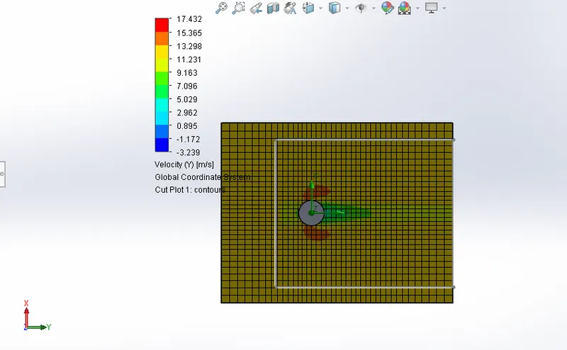
Fig. Velocity Plot for a simulation.
8) Then by Clicking Animation option select wizard option ; animation time is put ,the next screen ask whether the model needs to be rotated during simulation.Next Screen asks whether we want to see flow field at particular instant or flow should continue till steady state is acheived.
9)The start and end point is then matched and control point is added to show results of cut plots .
Results:-
For Baseline Reynolds No
Velocity Cut-Plot
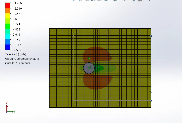
Fig .Velocity Plot for baseline Reynolds No
Observations:-
1)As the fluid moves over periphery of cylinder boundary layer is formed at the central layer and due to adverse pressure gradient flow gets seperated into wake or turbulences.
2)Velocity is maximum at the central part of the cylinder while due to flow seperation low velocity flow is observed behind the component.
Pressure Cut Plot
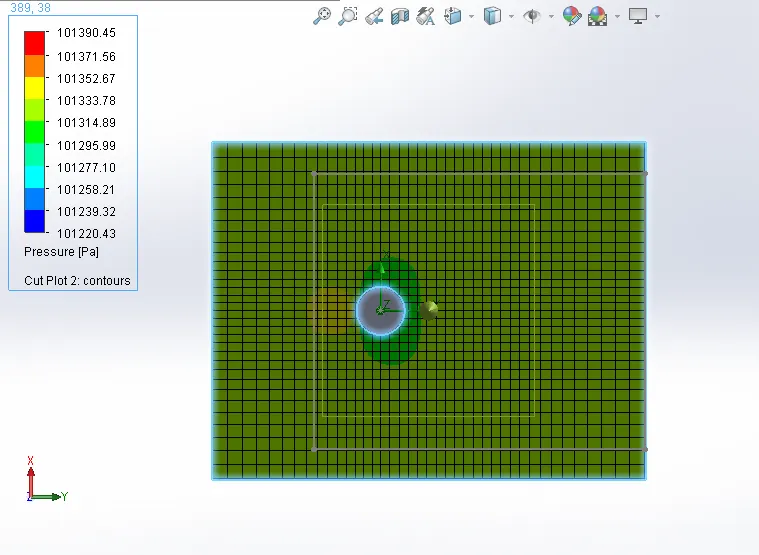
Fig. Pressure Plot for Baseline Reynolds No.
Observations:-
1) Back pressure is built at inlet due to change in direction of flow ,also as boundary layer seperates low pressure region is formed around centre.
1)Velocity Animation for Baseline Reynolds Number
2)Pressure Distribution For base line Reynolds Number
For Reynolds No. Increment of 20%
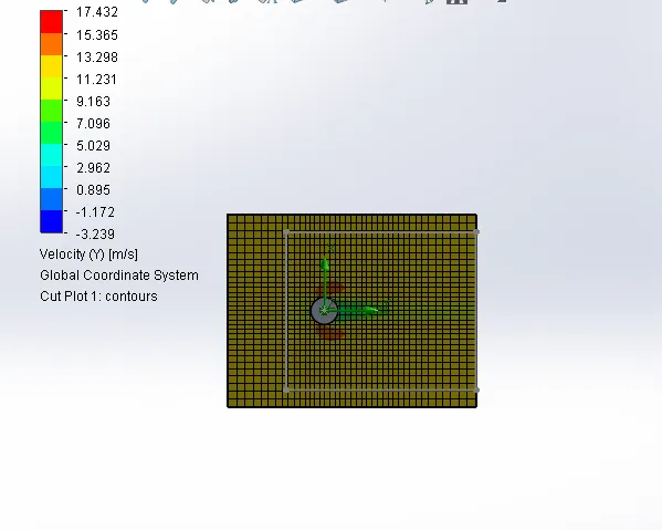
Fig.Velocity Cut-plot for Reynolds No. Increment of 20%
Observation:-
1) As the velocity is increased the turbulence is acheived even prior before then acheived earlier.Also vortices are formed at the end before the flow is converged.
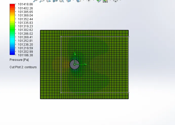
Fig.Pressure Cut-Plot for 20% increment in Reynolds No.
1)Velocity Animation for Reynolds Number increment of 20%
2)Pressure Distribution for increment of 20% Reynolds No
For Reynolds No. increment of 40%
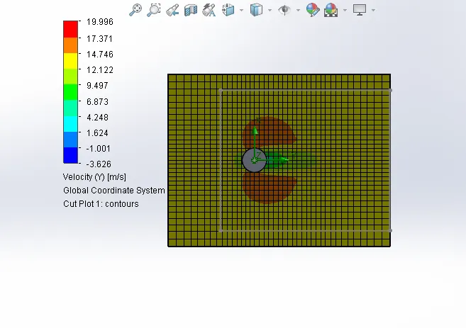
Fig.Velocity Cut-Plot for Reynolds No increment of 40%
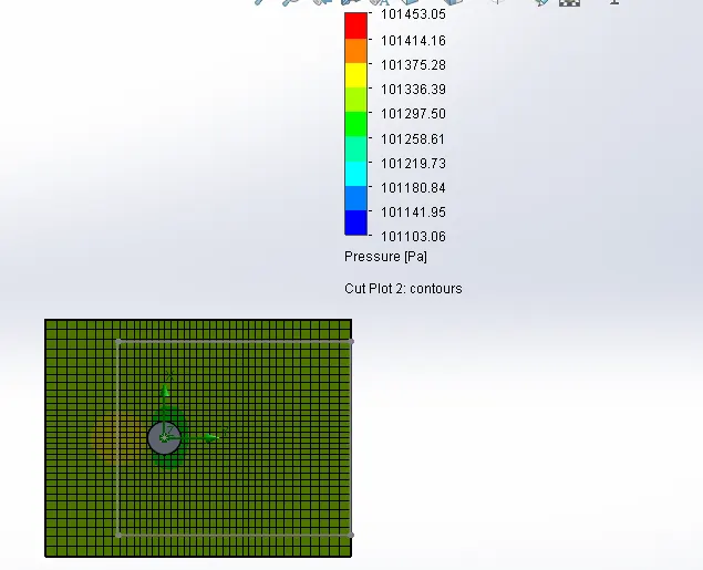
Fig.Pressure Cut-Plot for Reynolds No. 40% Increment
1)Velocity Animation for Reynolds No increment of 40%
2)Pressure Distriution for Reynolds No increment of 40%
For Reynolds No. increment by 100%
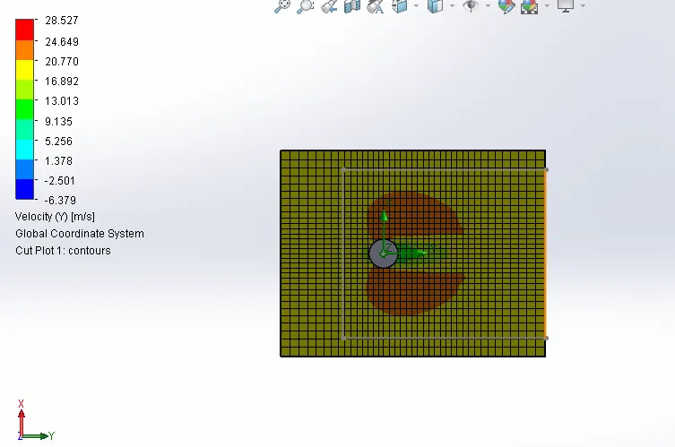
Fig.Velocity Cut-Plot for Reynolds No Increment of 100%
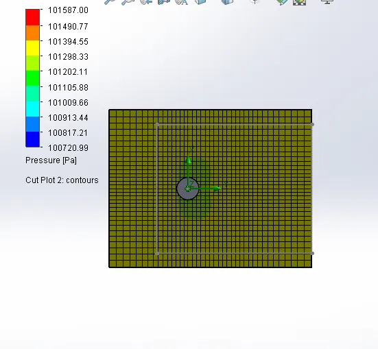
Fig.Pressure Cut-Plot for Reynolds No Increment of 100%
1)Velocity Animation for Reynolds No increment of 100%
2)Pressure Distribution for Reynolds No Increment of 100%
Conclusion:-
1)As velocity increases the flow achieve turbulence very quickly; vortices are formed at the end of domain.
2)There is pressure drop in each case at right side of the cylinder due to adverse pressure gradient creating a low pressure zone there;which is similar as developed in case of aerofoil.