Final Project: Electric Rickshaw modelling
INTRODUCTION
- Electric rickshaws(also known as electric tuk-tuks or e-rickshaws or toto or e-tricycles) have been becoming more popular in some cities since 2008 as an alternative to auto rickshaws and pulled rickshaws because of their low fuel cost, and less human effort compared to pulled rickshaws.
- They are being widely accepted as an alternative to petrol/diesel/CNG auto rickshaws. They are three-wheelers powered by an electric motor ranging from 650 to 1400 Watts.
- They are mostly manufactured in India and China, only a few other countries manufacture these vehicles.
- Here, the e-rickshaw is designed in CREO and MATLAB simulink. In the designed electric rickshaw main blocks are battery, drive cycle, controlled DC motor, vehicle body and transmission system. Drive cycle is the input of human effort that how the driver is going to drive the vehicle actually. We can use drive cycles like FTP75, WOT or by using excel.
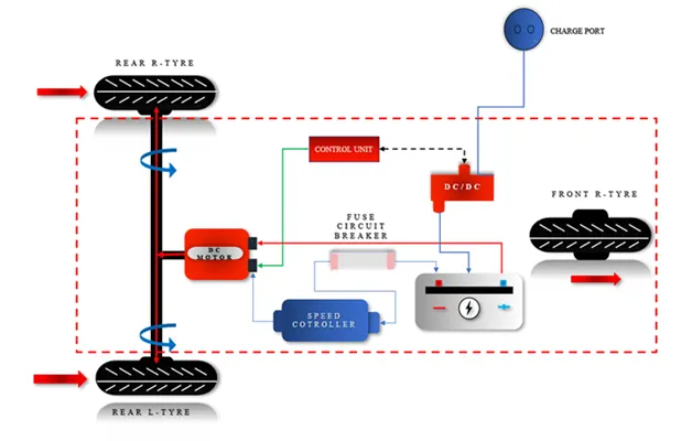
- The main objective of this project is to obtain the speed by the driver, to estimate the temperature of motor and the controller, to estimate the state of charge and distance travelled by the vehicle.
CONSTRUCTION OF ELECTRIC RICKSHAW:
- Electric rickshaws are extremely lightweight, and have a mild steel tubular chassis, consisting of three wheels. They use a brushless direct current motor.
- Electric rickshaws can vary based on body and design depending on if it is a load carrier, which can carry up to 500-1000 kg, or a passenger vehicle. It can vary all the way from having no roof to a full body with windshield and other facilities for the driver and passengers.
- They are also distinguished based on the controller unit, and voltage supplied by it and its current output; the electrical system used in the Indian version is 48V.
- The weight of the electric rickshaws differs as well depending on the model, but for the most part, they are extremely lightweight.
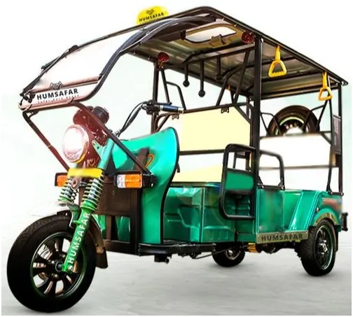
General Details of Electric Rickshaw:
- Battery Type Lithium Ion 330V 75Ah
- Vehicle Kerb weight 260Kgs
- Load Capacity 340Kgs
- Vehicle Speed 7 Kmph
- Driving Range 140Km
- Number of wheels per axle is 2
- Frontal Area 91m
- Drag coefficient 5
- Wheel Radius 306m
- Vertical Load 3000N
- Nominal Voltage 330V
- Rated Capacity 75Ah
- Initial SOC 100%
- Internal Resistance 5 ohm
PROCEDURE:
- Vehicle Body Subsystem Model:
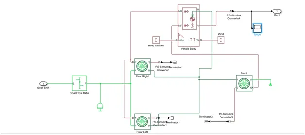
- The block accounts for body mass, aerodynamic drag, road incline, and weight distribution between axles due to acceleration and road profile. The vehicle can have the same or a different number of wheels on each axle.
- Connection H is the mechanical translational conserving port associated with the horizontal motion of the vehicle body. The resulting traction motion developed by tires should be connected to this port.
- Connections V, NF, and NR are physical signal output ports for vehicle velocity and front and rear normal wheel forces, respectively. Wheel forces are considered positive if acting downwards. Connections W and beta are physical signal input ports corresponding to headwind speed and road inclination angle, respectively.
VEHICLE BODY PARAMETERS:
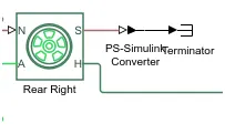
- Represents the longitudinal behavior of a highway tire characterized by the tire magic formula. The block is built from Tire- Road Interaction and simscape foundation.
- Connection A is the mechanical rotational conserving port for the wheel axle. Connection H is the mechanical translational conserving port for the wheel hub through which the thrust developed by the tire is applied to the vehicle.
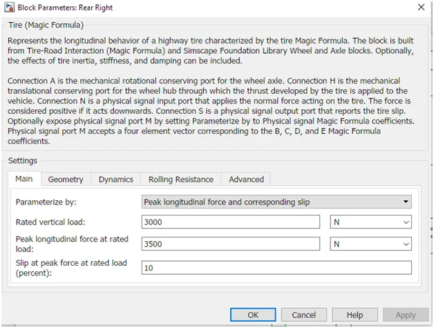
- Connection N is a physical signal input port that applies the normal force acting on the tire. The force is considered positive if it acts downwards. Connection S is a physical signal output port that reports the tire slip.
GEAR:
- Represents a fixed-ratio gear or gear box. No inertia or compliance is modeled in this block. You can optionally include gear meshing and viscous bearing losses.
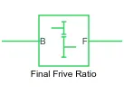
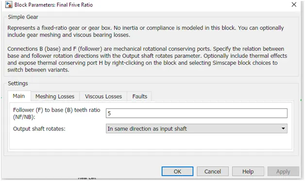
- Connections B (base) and F (follower) are mechanical rotational conserving ports. Specify the relation between base and follower rotation directions with the Output shaft rotates parameter. Optionally include thermal effects and expose thermal conserving port H by right-clicking on the block and selecting Simscape block choices to switch between variants.
VEHICLE BODY:
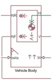
- Represents a two-axle vehicle body in longitudinal motion. The block accounts for body mass, aerodynamic drag, road incline, and weight distribution between axles due to acceleration and road profile.
- The vehicle can have the same or a different number of wheels on each axle. Optionally include pitch and suspension dynamics or additional variable mass and inertia. The vehicle does not move vertically relative to the ground.
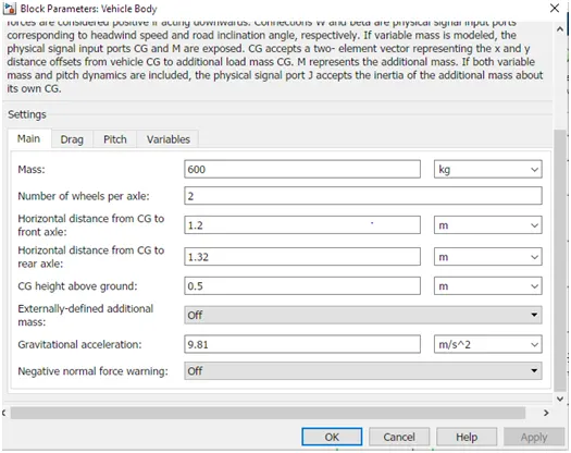
- Connection H is the mechanical translational conserving port associated with the horizontal motion of the vehicle body. The resulting traction motion developed by tires should be connected to this port. Connections V, NF, and NR are physical signal output ports for vehicle velocity and front and rear normal wheel forces, respectively. Wheel forces are considered positive if acting downwards.
- Connections W and beta are physical signal input ports corresponding to headwind speed and road inclination angle, respectively. If variable mass is modeled, the physical signal input ports CG and M are exposed. CG accepts a two- element vector representing the x and y distance offsets from vehicle CG to additional load mass CG. M represents the additional mass. If both variable mass and pitch dynamics are included, the physical signal port J accepts the inertia of the additional mass about its own CG.
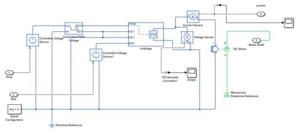
MOTOR AND POWER CONVERTER SUBSYSTEM:
H-BRIDGE:
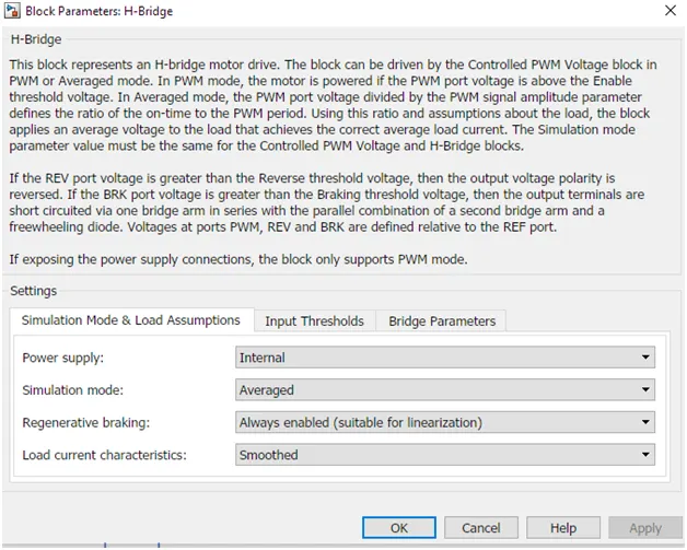
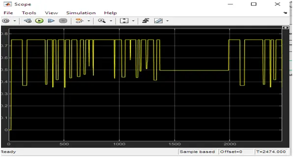
- This block represents an H-bridge motor drive. The block can be driven by the controlled PWM voltage block in PWM or Averaged Mode.
- In PMW mode, the motor is powered if the PWM port voltage is above the enabled threshold voltage.
- In Averaged mode, the PMW port voltage divided by the signal amplitude parameter defines the ratio of On-time to the PWM period.
- Connection REF is for the reference input. This combined with the PWM connected will form the pulse input for the H-bridge.
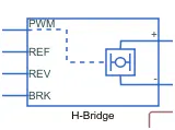
- Connection REV corresponds to the reverse motion of the motor which means, the backward motion of the vehicle.
- Connection BRK is for the braking of the vehicle.
- Since, the PWM mode results in a huge amount of simulation time,Averaged mode is selected for this simulation.
- Load current characteristics are considered to be smoothed here.
- The brake input is connected to the Controlled Voltage Source. This will generate emf corresponding to the intensity of brakes applied and fed the power back to the battery.
DC-MOTOR:
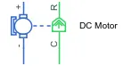
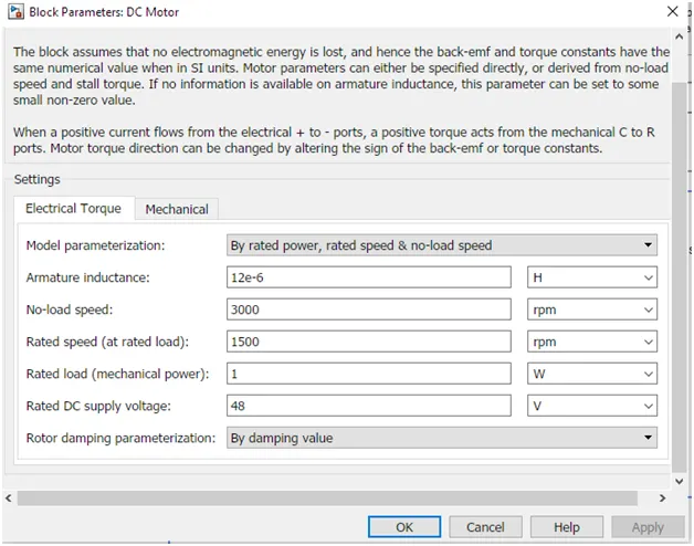
- This block represents the electrical and torque characteristics of a DC motor.
- The block assumes that no electromagnetic energy is lost, and hence the back-emf and torque constants have the same numerical value when in SI units. Motor parameters can either be specified directly, or derived from no-load speed and stall torque. If no information is available on armature inductance, this parameter can be set to some small non-zero value.
- When a positive current flows from the electrical + to - ports, a positive torque acts from the mechanical C to R ports. Motor torque direction can be changed by altering the sign of the back-emf or torque constants.
CONTROLLED PWM VOLTAGE:
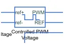
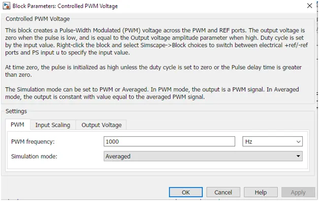
- This block creates a Pulse-Width Modulated (PWM) voltage across the PWM and REF ports. The output voltage is zero when the pulse is low, and is equal to the Output voltage amplitude parameter when high. Duty cycle is set by the input value. Right-click the block and select Simscape->Block choices to switch between electrical +ref/-ref ports and PS input u to specify the input value.
- At time zero, the pulse is initialized as high unless the duty cycle is set to zero or the Pulse delay time is greater than zero.
- The Simulation mode can be set to PWM or Averaged. In PWM mode, the output is a PWM signal. In Averaged mode, the output is constant with value equal to the averaged PWM signal.
3. LONGITUDINAL DRIVE:
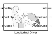
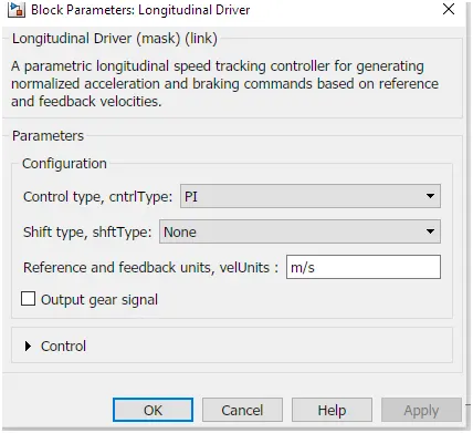
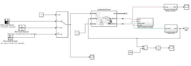
- Longitudinal driver is an inbuilt block provided by the powertrain blockset.
- It is a parametric longitudinal speed tracking controller for generating normalized Accleration and Braking commands based on reference and feedback velocities.
- The VelRef port is the reference velocity port where the input driver cycle data is fed.
- The VelFdbk port corresponds to the feedback velocity. The actual velocity output given by the vehicle body is connected here. By comparing the actual velocity with the reference velocity, the driver block generates acceleration and braking signals in order to minimize the error between the two concerned velocities.
- The selected control type is PI. Accordingly, the block implements the proportional- integral control with tracking windup and feed-forwards gains.
- BATTERY STATE OF CHARGE:
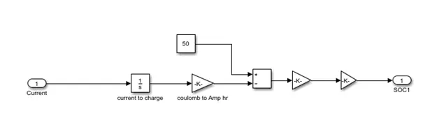
- A small subsystem is created to calculate the state of charge of the battery.
- This subsystem takes the battery current as input.
- The essential process to calculate the SOC is by subtracting the charge from the rated capacity of the battery.
- The current is integrated w.r.t time to get the charge in coulombs. Now, this coulomb is modified in to Ampere hours.
- The value obtained is now subtracted from the charging capacity of the battery. 50Ah.
- The remaining charge is now converted into percentage value of the charging capacity of the battery.
- REFERENCE VELOCITY STYLE:
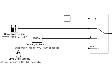
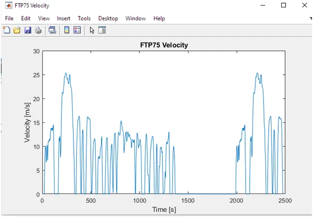
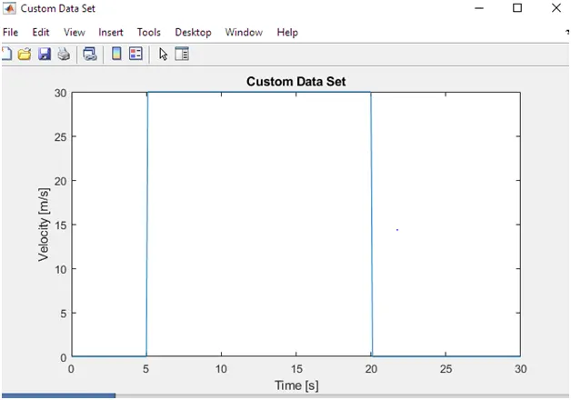
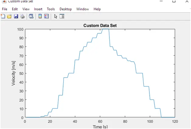
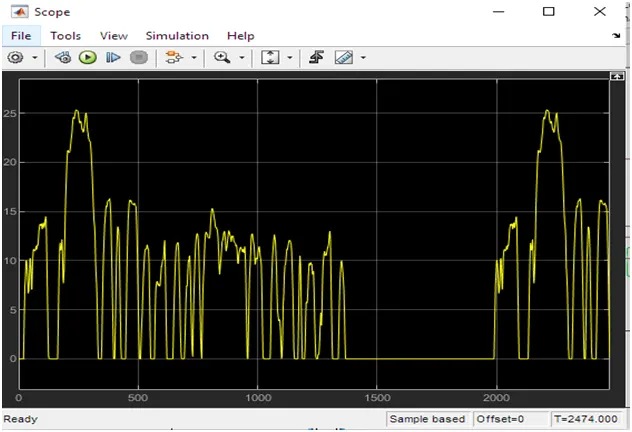
- Drive cycle is assumed to be the driver’s input of a vehicle. I have used three drive cycles which is used to test the vehicle performance. These drive cycle will have high speed, low speed, braking conditions in it.
- There are different drive cycles like WOT, FTP75. Here in this model I have used FTP75, WOT and Manually prepared in excel drive cycle source.
FTP75:
WOT:
MANUAL DRIVE CYCLE:
Attaching the drive cycle excel sheet with this model.
SIMULINK MODEL:
RESULT:
REFERENCE SPEED:
MOTOR VOLTAGE:
DISTANCE COVERED:
STATE OF CHARGE:
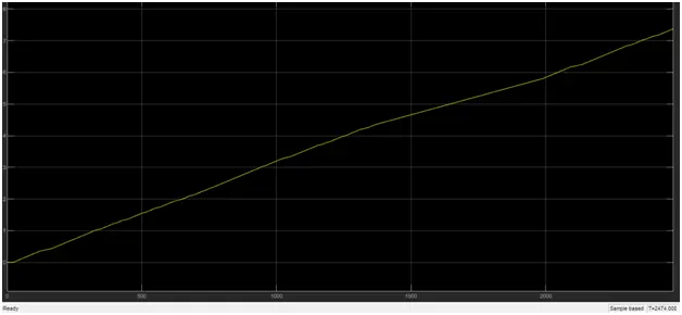
- The distance covered is approximately 19Kms. The model is run for 2474 seconds.
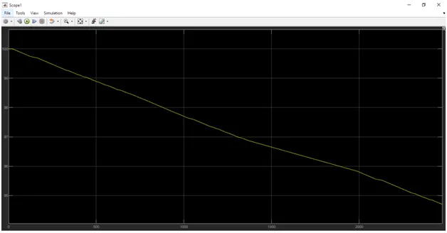
- The state of charge of the battery decreases as the simulation is in progress from 100% to 93%.
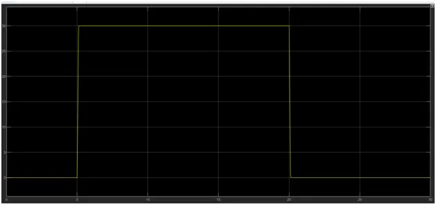
WIDE OPEN THROTTLE:
REFERENCE VOLTAGE:
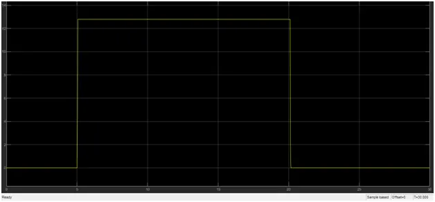
MOTOR VOLTAGE:
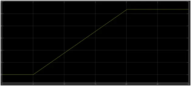
DISTANCE COVERED:
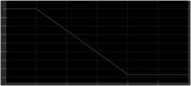
SOC:
- The distance covered for the duration of 30s is 5kms.
- The battery voltage decreases from 100% to 98%.
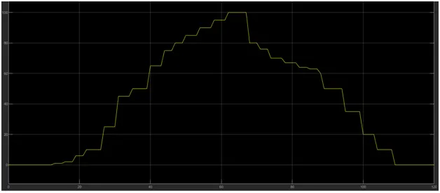
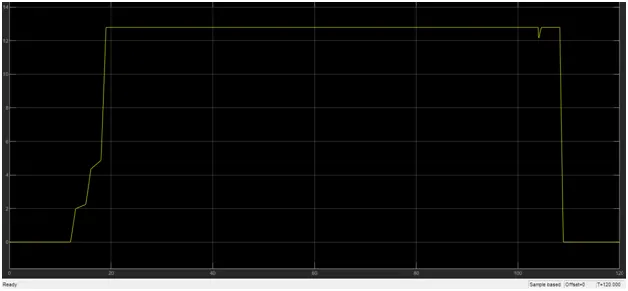
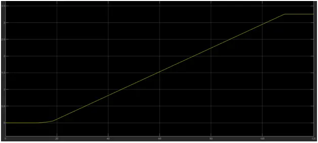
FOR MANUALLY PREPARED DRIVE CYCLE:
REFERENCE VOLTAGE:
MOTOR VOLTAGE:
DISTANCE COVERED:
SOC:
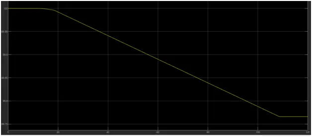
- The distance covered is 3.5Kms in 120 seconds.
- The battery charge decreases from 100% to 98% in 120 seconds.
CONCLUSION:
- The model was successfully run for simulation under the standard FTP75 cycle, WOT and Manual drive cycle. The results have been properly analyzed.