Final Project: Electric Rickshaw modelling
MATLAB model of an electric rickshaw (three wheel passenger vehicle)
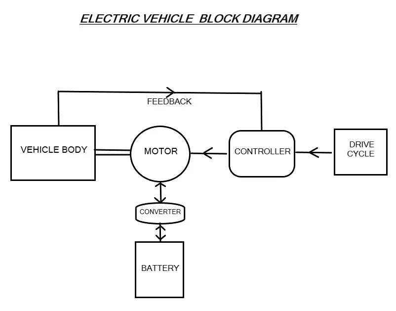
Below is the block diagram of the Electric rickshaw Model,
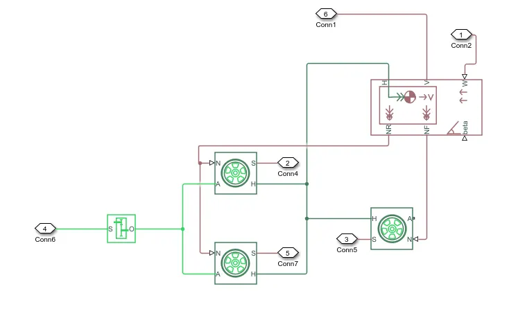
Below the Simulink model of the Vehicle,which consists of the 3 wheels along with the vehicle body and gear box.This vehicle body is connected in between front and rear wheels as shown in the below model.
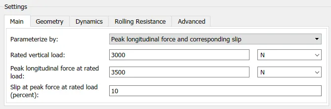
For the tire block,connection A is the mechanical rotational conserving port for the wheel axle. Connection H is the mechanical translational conserving port for the wheel hub through which the thrust developed by the tire is applied to the vehicle. Connection N is a physical signal input port that applies the normal force acting on the tire. The force is considered positive if it acts downwards. Connection S is a physical signal output port that reports the tire slip. Optionally expose physical signal port M by setting Parameterize by to Physical signal Magic Formula coefficients. Physical signal port M accepts a four element vector corresponding to the B, C, D, and E Magic Formula coefficients.Now coming to the parameters of the wheel in the below diagram we can see that rated vertical load is 3000N, and the peak longitudinal force is 3500N. % slip at peak force is set to 10. In the geometry of the wheel rolling radius is set to 0.3m. In dynamics block inertia we are ignoring and rolling resistance is set to zero.The velocity of the threshold is 0.1m/s.
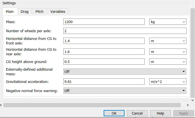
In the vehicle body blocks parameters are configured as shown in the below diagram.A two-axle vehicle body in longitudinal motion. The block accounts for body mass, aerodynamic drag, road incline, anhicled weight distribution between axles due to acceleration and road profile. The vehicle can have the same or a different number of wheels on each axle. Optionally include pitch and suspension dynamics or additional variable mass and inertia. The vehicle does not move vertically relative to the ground.Connection H is the mechanical translational conserving port associated with the horizontal motion of the vehicle body. The resulting traction motion developed by tires should be connected to this port. Connections V, NF, and NR are physical signal output ports for vehicle velocity and front and rear normal wheel forces, respectively. Wheel forces are considered positive if acting downwards. Connections W and beta are physical signal input ports corresponding to headwind speed and road inclination angle, respectively. If variable mass is modeled, the physical signal input ports CG and M are exposed. CG accepts a two- element vector representing the x and y distance offsets from vehicle CG to additional load mass CG. M represents the additional mass. If both variable mass and pitch dynamics are included, the physical signal port J accepts the inertia of the additional mass about its own CG.
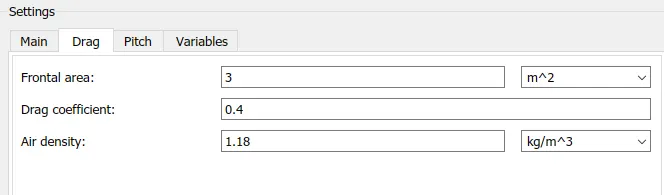
additionally the drag force parameters are taken as shown in the below,frontal area is 3 m^3,drag coefficient 0.4 and air density to be 1.18 kg/m^3
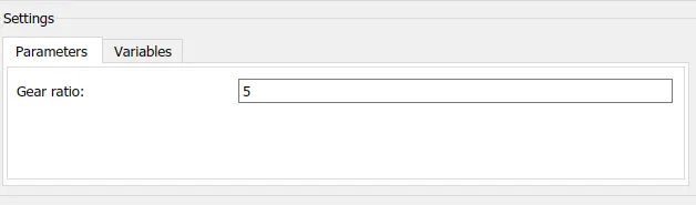
Gear Box:Block represents an ideal, non-planetary, fixed gear ratio gear box. The gear box is characterized by its only parameter, Gear ratio, which can be positive or negative. Connections S and O are mechanical rotational conserving ports associated with the box input and output shaft, respectively. The gear ratio is determined as the ratio of the input shaft angular velocity to that of the output shaft.The gear ratio is set to 5.
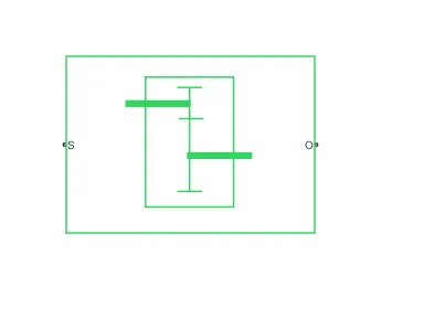
The block generates torque in positive direction if a positive torque is applied to the input shaft and the ratio is assigned a positive value.
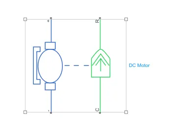
Motor:This vehicle is driven by the dc motor which is the PM brushed type motor.This block represents the electrical and torque characteristics of a DC motor.The block assumes that no electromagnetic energy is lost, and hence the back-emf and torque constants have the same numerical value when in SI units. Motor parameters can either be specified directly, or derived from no-load speed and stall torque. If no information is available on armature inductance, this parameter can be set to some small non-zero value.When a positive current flows from the electrical + to - ports, a positive torque acts from the mechanical C to R ports. Motor torque direction can be changed by altering the sign of the back-emf or torque constants.
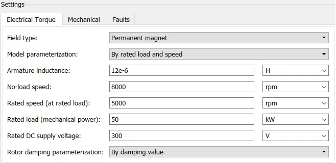
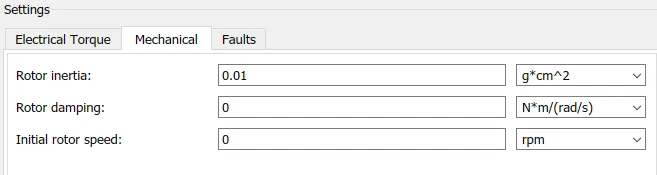
Now about motor parameters, La is taken to be 12*10^-6 H,noload speed to be 8000 rpm,rated speed as 5000 rpm, dc supply voltage as 300 V, rotor inertia to be 0.01 g*cm^2
Motor Controller:The motor controller will get the input from longitudinal driver.It controls the speed of the motor and the driver according to the driver input.We have two main parts named PWM voltage generator and H-Bridge. acclemd of a longitudinal driver is connected to ref+ of controlled PWM voltage, and ref- is grounded.Similarly the H-bridge inputs PWM is connected to the PWM output of the Controlled PWM block and REF is connected to the REF output of the Controlled PWM block. This H-bridge inturn feeds the dc motor.
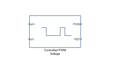
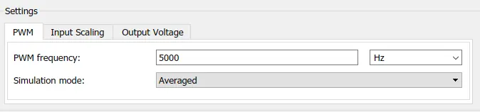
Controlled PWM Voltage block creates a Pulse-Width Modulated (PWM) voltage across the PWM and REF ports. The output voltage is zero when the pulse is low, and is equal to the Output voltage amplitude parameter when high. Duty cycle is set by the input value. Right-click the block and select Simscape->Block choices to switch between electrical +ref/-ref ports and PS input u to specify the input value.At time zero, the pulse is initialized as high unless the duty cycle is set to zero or the Pulse delay time is greater than zero.The Simulation mode can be set to PWM or Averaged. In PWM mode, the output is a PWM signal. In Averaged mode, the output is constant with value equal to the averaged PWM signal.PWM frequency is taken as 5000 Hz and simulation mode is set to Averaged.Output voltage is 300V.
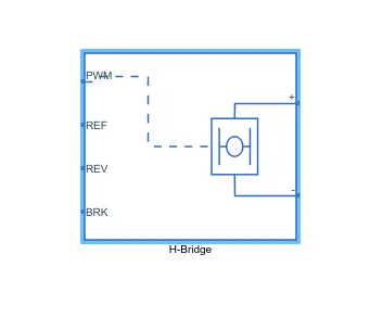
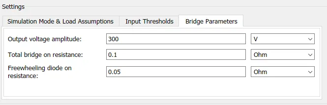
Above block represents an H-bridge motor drive. The block can be driven by the Controlled PWM Voltage block in PWM or Averaged mode. In PWM mode, the motor is powered if the PWM port voltage is above the Enable threshold voltage. In Averaged mode, the PWM port voltage divided by the PWM signal amplitude parameter defines the ratio of the on-time to the PWM period. Using this ratio and assumptions about the load, the block applies an average voltage to the load that achieves the correct average load current. The Simulation mode parameter value must be the same for the Controlled PWM Voltage and H-Bridge blocks.If the REV port voltage is greater than the Reverse threshold voltage, then the output voltage polarity is reversed. If the BRK port voltage is greater than the Braking threshold voltage, then the output terminals are short circuited via one bridge arm in series with the parallel combination of a second bridge arm and a freewheeling diode. Voltages at ports PWM, REV and BRK are defined relative to the REF port.If exposing the power supply connections, the block only supports PWM mode.Below is the H-bridge parameters.The output voltage amplitude is 300 V.
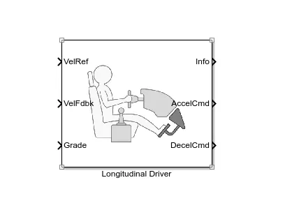
Longitudinal Driver:A parametric longitudinal speed tracking controller for generating normalized acceleration and braking commands based on reference and feedback velocities.Use the external actions to input signals that can disable, hold, or override the closed-loop commands determined by the block. The block uses this priority for the input commands: disable, hold, override.The control is chosen as PI controller.
Drive Cycle:Generates a standard or user-specified longitudinal drive cycle. The block output is the vehicle longitudinal speed. You can import drive cycles from:
- Predefined sources
- Workspace variables, including arrays and time series objects
- mat, xls, xlsx, or txt files
Use the fault tracking parameters to identify drive cycle faults within specified speed and time tolerances.
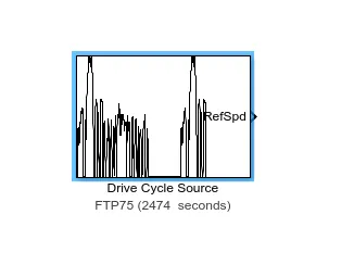
Here we have chosen FTP75 drive cycle.
Results:
By running the vehicle with FTP75 drive cycle for 2474 seconds the distance travelled is 5.667 kmph.Below is the complete simulation model of the Electric Rickshaw.
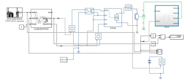
Below is the FTP74 Drive cycle output:

Below is the actual velocity of the vehicle output:

Below is the accleration command output:

Now we will consider the WOT Drive cycle with the following parameters
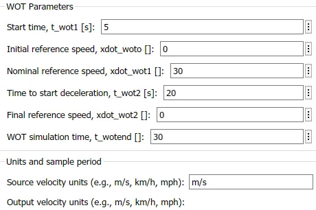
By running the vehicle with WOT drive cycle for 30 seconds the distance travelled is 0.1191 kmph.Below is the complete simulation model of the Electric Rickshaw
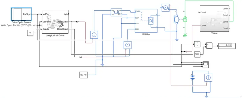
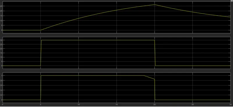
Plot of the Drive cycle ,velocity of the rickshaw and the accleration command is as shown in the below attachment.