Final Project: Electric Rickshaw modelling

 Q. CREATE A DETAILED MATLAB MODEL OF AN ELECTRIC RICKSHAW (THREE WHEEL PASSENGER VEHICLE) AS PER DETAILS BELOW:-

REAR WHEELS DRIVEN BY PM BRUSHED TYPE MOTOR

ASSUME EFFICIENCY POINTS OF MOTOR CONTROLLER AND MOTOR

MAKE AN EXCEL SHEET OF ALL INPUT AND ASSUMED DATA

RESULTS: FOR ANY THREE STANDARD DRIVING CYCLES SHOW ENERGY CONSUMPTION, TEMPERATURE RISE OF MOTOR AND CONTROLLER FOR 100KM CONSTANT SPEED DRIVING AT 45KMPH.

AIM OF THE PROJECT:- TO DESIGN AN ELECTRIC RICKSHAW IN MATLAB AND FORM 3 INPUTS WITH RESULTS OF ENERGY CONSUMPTION, TEMPERATURE RISE OF MOTOR AND CONTROLLER FOR 100KM CONSTANT SPEED DRIVING AT 45KMPH.

SOLUTION:-

THEORY:-

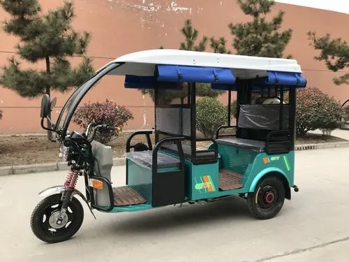
Electric rickshaws have been becoming more popular in some cities since 2008 as an alternative to auto rickshaws and pulled rickshaws because of their low fuel cost, and less human effort compared to pulled rickshaws. They are being widely accepted as an alternative to petrol/diesel/CNG auto rickshaws. They are three-wheelers powered by an electric motor ranging from 650 to 1400  Watts. They are mostly manufactured in India and China, only a few other countries manufacture these vehicles. Battery-run rickshaws could be a low-emitter complementary transport for the low-income people, who suffer most from a lack of transport facility, if introduced in a systematic manner according to experts.

These rickshaws have a M.S(Mild Steel) tubular Chassis, consisting of three wheels with a differential mechanism at the rear wheels. The motor is brushless DC motor manufactured mostly in India and China. The electrical system used in Indian version is 48V and Bangladesh is 60V. The body design from most popular Chinese version is of very thin iron or aluminium sheets. Vehicles made in fibre are also popular because of their strength and durability, resulting in low maintenance, especially in India. Body design is varied from load carriers, passenger vehicles with no roof, to full body with windshield for drivers comfort. It consist of a controller unit. They are sold on the basis of voltage supplied and current output, also the number of mosfet (metal oxide field effect transistors) used. The battery used is mostly lead acid battery with life of 6–12 months. Deep cycle batteries designed for electric vehicles are rarely used. Weight of the electric car has also been a recurring design difficulty in them.

MODEL:-

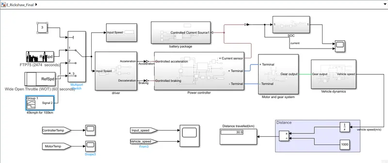
BLOCKS CONTENT:-

MODEL

S.NO	NAME OF BLOCK	NUMBER OF BLOCKS
1.	Constant	2
2.	Drive cycle	2
3.	Signal builder	1
4.	Multiport switch	1
5.	From block	1
6.	Driver subsystem	1
7.	S-PS converter	2
8.	Power controller subsystem	1
9.	PS-S converter	1
10.	SOC subsytem	1
11.	Motor and gear subsystem	1
12.	Vehicle dynamics	1
13.	Scope	1
14.	Display	1
15.	Product	1
16.	Integrator	1

DRIVER SUBSYSTEM

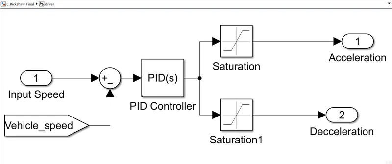
S.NO	NAME OF BLOCK	NUMBER OF BLOCKS
1.	From(vehicle-speed)	1
2.	Sum	1
3.	PID controller	1
4.	Saturation(acceleration&deacceleration)	2

BATTERY PACKAGE

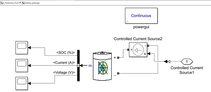
S.NO	NAME OF BLOCK	NUMBER OF BLOCKS
1.	Continuous powergui	1
2.	Scope	3
3.	li-ion battery	1
4.	Controlled current source	1
5.	PS-S converter	1

POWER CONTROLLER SUBSYSTEM

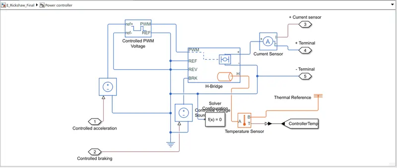
S.NO	NAME OF BLOCK	NUMBER OF BLOCKS
1.	Controlled voltage source	2
2.	Controlled PWM voltage	1
3.	H-bridge with thermal on	1
4.	Solver configuration	1
5.	Temperature configuration	1
6.	Current sensor	1
7.	Thermal reference	1
8.	PS-S converter	1
9.	Goto(controller temp)

SOC SUBSYSTEM

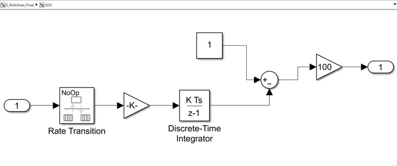
S.NO	NAME OF BLOCK	NUMBER OF BLOCKS
1.	Rate transition	1
2.	Gain	2
3.	Discrete-time integrator	1
4.	Constant	1
5.	Sum	1

MOTOR AND GEAR SYSTEM SUBSYSTEM

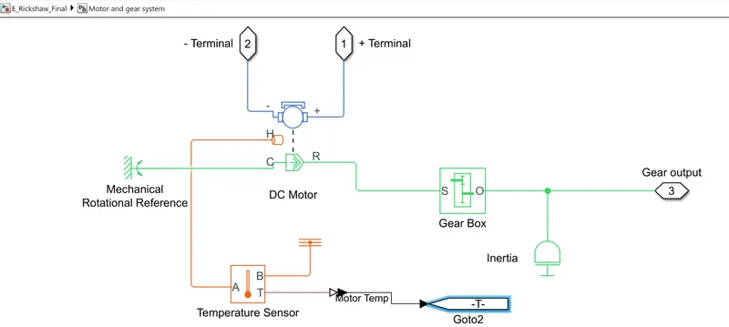
S.NO	NAME OF BLOCK	NUMBER OF BLOCKS
1.	Dc motor with thermal on	1
2.	Mechanical rotational reference	1
3.	Temperature sensor	1
4.	Thermal reference	1
5.	PS-S converter	1
6.	Gear box	1
7.	Inertia	1
8.	Goto T	1

VEHICLE DYNAMICS

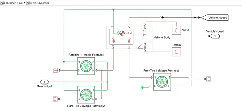
S.NO	NAME OF BLOCK	NUMBER OF BLOCKS
1.	Tire	3
2.	Vehicle body	1
3.	Goto(vehicle speed)	1
4.	PS Terminator	1

Assumed Input Data:

Sr No.	Name of the Block	Input Data
1	Longitudinal Driver
1.1	Control type	PI
1.2	Shift Type	None
2	Battery Subsystem
2.1	Battery Type	Li-ion
2.2	Controlled Current Source	Default inputs
2.3	Nominal voltage (V)	48
2.4	Rated capacity (Ah)	153.54
2.5	Initial state-of-charge (%)	100
2.6	Battery response time (s)	30
3	DC Motor Subsystem
3.1	Controlled PWM Voltage Block
3.1.1	PWM Frequency (Hz)	4000
3.1.2	Simulation Mode	Averaged
3.1.3	Sample Time (s)	1e-6
3.1.4	Output voltage amplitude (V)	5
3.2	DC Motor Block
3.2.1	Field type	Permanent Magnet
3.2.2	Model parameterization	By rated load and speed
3.2.3	Armature inductance (uH)	34
3.2.4	No-load speed (rpm)	4800
3.2.5	Rated speed (at rated load) (rpm)	3855
3.2.6	Rated load (mechanical power) (kW)	8
3.2.7	Rated DC supply voltage (V)	48
3.2.8	Rotor damping parameterization	By damping value
3.2.9	Rotor inertia (g*cm^2)	0.01
3.2.10	Rotor damping (N*m/(rad/s))	0
3.2.11	Initial rotor speed	0
4	Vehicle Body Subsystem
4.1	Gearbox
4.1.1	Follower (F) to base (B) teeth ratio (NF/NB)	7.2
4.1.2	Output shaft rotates	In same direction as input shaft
4.2	Tire (Magic Formula) (Same for all three tires)
4.2.1	Main	Default values
4.2.2	Geometry
4.2.3	Rolling radius (m)	0.254
4.3	Vehicle Body Block
4.3.1	Mass (kg)	600
4.3.2	Number of wheels per axle	2
4.3.3	Horizontal distance from CG to front axle (m)	1.4
4.3.4	Horizontal distance from CG to rear axle (m)	1.6
4.3.5	CG height above ground (m)	0.25
4.3.6	Externally-defined additional mass	Off
4.3.7	Gravitational acceleration (m/s^2)	9.81
4.3.8	Negative normal force warning	Off
4.3.9	Drag
4.3.10	Frontal area (m^2)	1.48
4.3.11	Drag coefficient	0.5
4.3.12	Air density (kg/m^3)	1.18

                              Table 2: Simulation Inputs

To model the three wheeled electric vehicle the above listed blocks are the basic blocks that consists of the powertrain, battery, and DC motor. The assumed input data is also discussed with the theory below and the inputs are mentioned in the table as above. This model is the basic model of any three wheel electric vehicle, a much advanced modelling will be needed further on to simulate an actual vehicle. The explanation of the modelling is as carried out below.

EV Model:

Constant Block:

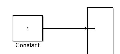This block is connected to the multiport switch to select the modes to decide which drive cycle source to be used for the simulation. For this model FTP 75 drive cycle, WOT drive cycle and a drive cycle made in an MS Excel sheet was taken into consideration for simulation.

Drive Cycle Source FTP 75:

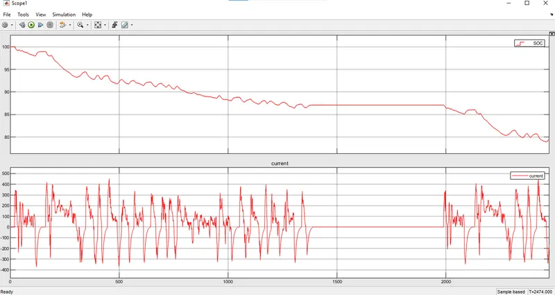
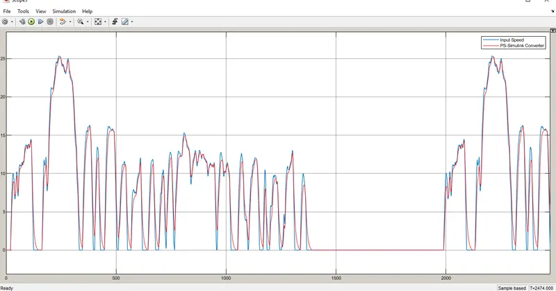
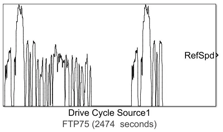FTP 75 drive cycle was considered to be simulated on this model, where the drive cycle was simulated for 2474 seconds and the output graphs were plotted for Temperature of DC motor and H-Bridge, SOC, current, speed from the drive cycle and vehicle speed and acceleration given by the longitudinal driver.

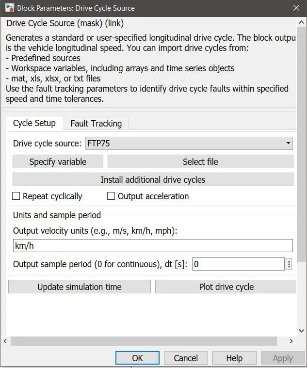
Drive Cycle Source WOT:

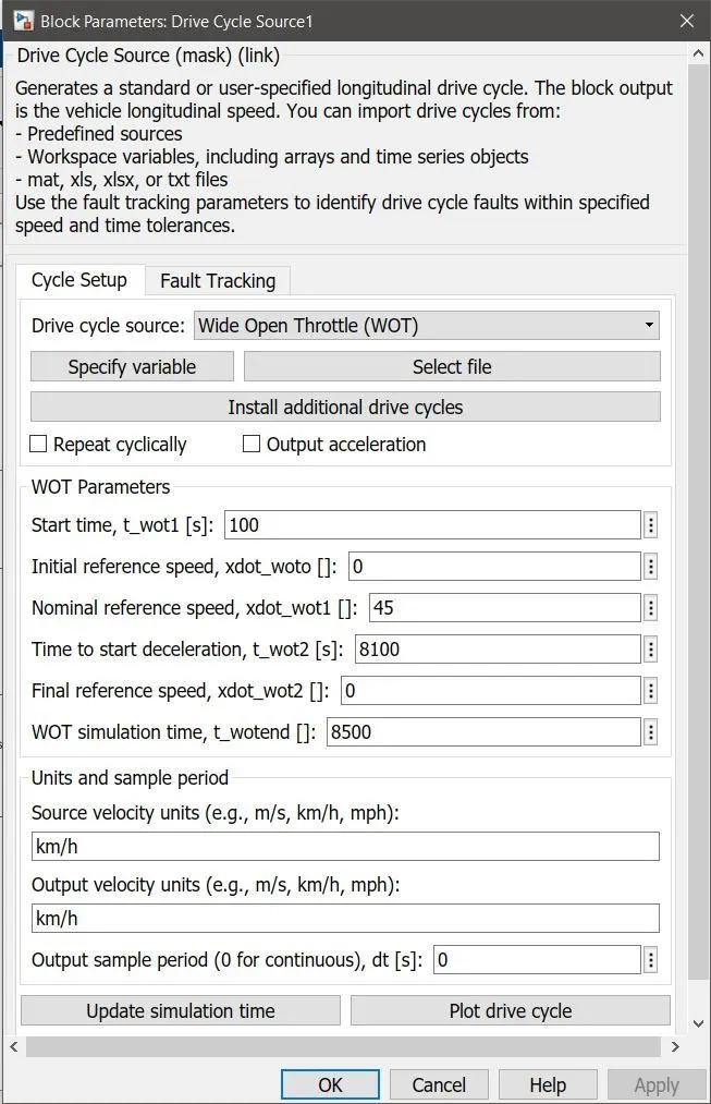
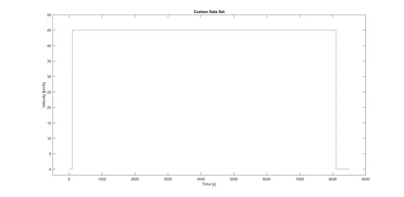
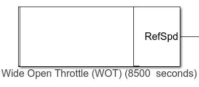 Shown is the drive cycle block where WOT was selected in the options and the WOT condition was modelled in the block where the parameters were set to the conditions given in the objectives which state that the vehicle should run for 100 km constant speed driving at 45 kmph. The parameters can be seen below with the drive cycle plotted.

From Spread Sheet:

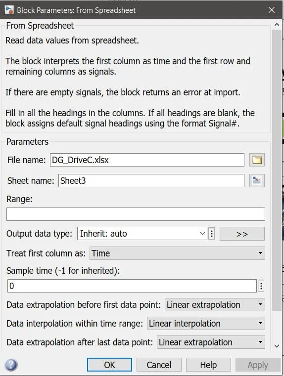
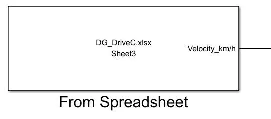 This block take inputs of Time and Velocity values available in the external spread sheet file to input the velocity values to the DC motor to propel the vehicle. This spread sheet was made by random velocity values in km/h for 500 seconds.

Multiport Switch:

 

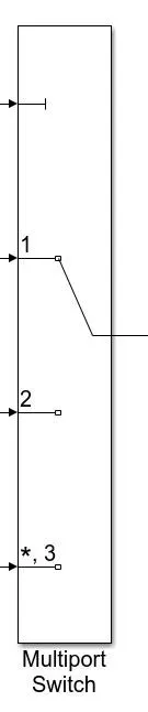
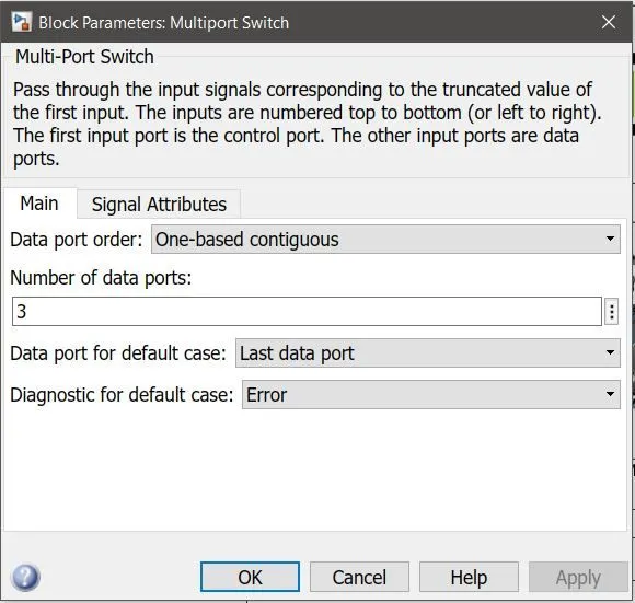
This switch acts as a selector switch to select what input has to be given further from multiple available input options. A constant block has to be connected to the top-most input port in this switch, where the connection number has to be input to select the input source. For this model three inputs were considered for simulation which were explained earlier.

 Control Type: This block implements proportional-integral (PI) control with tracking windup and feed-forward gains.

Reference and feedback unit: km/h

Connection Ports:

VelRef: This is the reference vehicle velocity which is connected to the result output speed scope it is in m/s.

VelFdbk: The vehicle velocity is connected to this port to get the feedback of the actual vehicle velocity from the vehicle body, which is further connected to the integrator.

Grade: Road grade angle is given to this connection with the help of a constant block. For this model no grade angle was considered for simulation.

Info: This is a bus signal which is an output port and is not considered for the simulation.

AccelCmd: This port is connected to the DC motor subsystem block to give acceleration command to the motor to propel the vehicle forward. This is connected to the controlled voltage source input signal with PS-Simulink converter .

DecelCmd: This port is again connected to the DC motor subsystem block to give the deceleration commands to the motor for the braking actions. This is connected to another controlled voltage source input with PS-Simulink converter, which is then connected to the BRK port of the H-bridge used in the DC motor subsystem.

Scope:

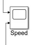There were in total four scope blocks used to get the simulation results. One to monitor the temperature rise of DC motor and H-Bridge, one for monitoring the state of charge (SOC%) of the battery used in the vehicle, one to analyse the voltage and current passed from battery to DC motor and the last one to monitor the velocity of the vehicle along with the drive cycle input.

Distance Calculation:

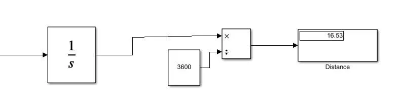
For distance calculation Integrator, Divide and Constant blocks were used to display the distance travelled by the vehicle.

Integrator: The output port of the vehicle body subsystem is connected to the integrator which basically gives the velocity output of the vehicle.

Divide: The output of the integrator is connected to the divide where it will be divided by the time to get the final distance output.

Time: A constant block was used to input the time. The time considered here is 3600 seconds.

Power GUI:

The powergui block allows you to choose one of these methods to solve your circuit:

• Continuous, which uses a variable-step solver from Simulink®
• Discretization of the electrical system for a solution at fixed time steps
• Continuous or discrete phasor solution

The powergui block also opens tools for steady-state and simulation results analysis and for advanced parameter design.

The configuration of the Solver tab depends on the option that you select from the Simulation type list.

Simulation type

Select Continuous ( default) to perform a continuous solution of the model.

Select Discrete to perform a discretization of the model. You specify the sample time in the Sample time parameter.

Select Phasor to perform continuous phasor simulation of the model, at the frequency specified by the Frequency (Hz) parameter.

If Simulation type is set to Discrete phasor, you can perform a phasor simulation at fixed time steps specified by the Sample time (s) parameter, at the frequency specified by the Frequency (Hz) parameter. The Discrete phasor solver uses simplified machine models that produce simulation results similar to transient stability software.

Sample time (s)

Specify the sample time used to discretize the electrical circuit. This parameter is visible only when the Simulation type parameter is set to Discrete or to Discrete phasor.

Set the Sample time parameter to a value greater than 0. The powergui block displays the value of the sample time. The default value is 50e-6 s.

Frequency (Hz)

Specify the frequency for performing the phasor simulation of the model. This parameter is enabled only when you set Simulation type to Phasor or to Discrete phasor. The powergui block displays the value of the phasor frequency. The default value is 60 Hz.

Battery Subsystem:

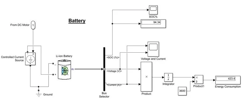
Below shown is the battery subsystem modelled for the vehicle.

Battery:

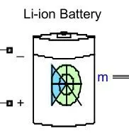
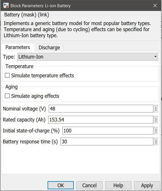
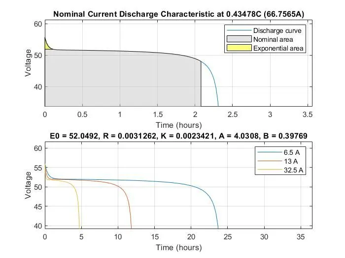
For this model a Li-ion battery was used, however, some inputs were changed for the vehicle application as shown below. This battery implements a generic battery model for most popular battery types. Temperature and aging (due to cycling) effects can be specified for Lithium-Ion battery type.

Battery Parameters:

SOC (State of Charge):

State of charge (SoC) is the level of charge of an electric battery relative to its capacity. The units of SoC are percentage points (0% = empty; 100% = full). An alternative form of the same measure is the depth of discharge (DoD), the inverse of SoC (100% = empty; 0% = full). SoC is normally used when discussing the current state of a battery in use, while DoD is most often seen when discussing the lifetime of the battery after repeated use.

In a battery electric vehicle (BEV), hybrid vehicle (HV), or plug-in hybrid electric vehicle (PHEV), SoC for the battery pack is the equivalent of a fuel gauge. It is important to mention that state of charge, presented as a gauge or percentual value at any vehicle dashboard, especially in plug-in hybrid vehicles, may not be representative for a real level of charge. In that particular case, some noticeable amount of energy stored in the electric battery is not shown at the dashboard, and it is reserved for hybrid-work operations. It permits a vehicle to accelerate with electric motor(s) mainly using battery energy, while engine serves as a generator is used to recharge the battery to the minimum level needed for such operation.

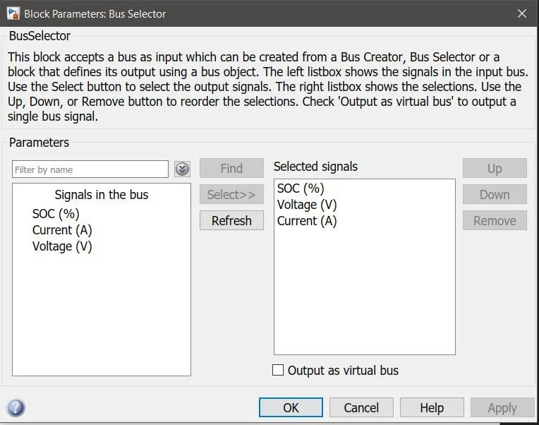
From the above selected Li-ion battery, we can determine SOC, voltage and current given to the DC motor through the battery by using the ‘Bus Selector’ block available in Simulink, where it selects and plots the determined for SOC, voltage and current and also can be displayed in numbers using display block and energy consumption can be calculated.

Bus Selector:

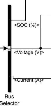
This block accepts a bus as input which can be created from a Bus Creator, Bus Selector or a block that defines its output using a bus object. The left listbox shows the signals in the input bus. Use the Select button to select the output signals. The right listbox shows the selections. Use the Up, Down, or Remove button to reorder the selections. Check 'Output as virtual bus' to output a single bus signal.

Controlled Current Source:

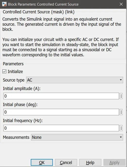
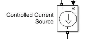 Converts the Simulink input signal into an equivalent current source. The generated current is driven by the input signal of the block. The parameters for this block were kept to its default values.

Electrical Ground:

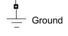 This block is the electrical ground block which is the ground to any electric circuit in Simulink, this block is connected to the negative terminal of the battery in this model.

Energy Consumption Calculation:

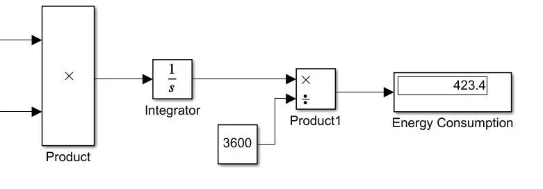
The energy consumption was calculating by taking a product of current and voltage given to DC motor and was integrated and divided by 3600 to get the consumption in Wh.

DC Motor Subsystem:

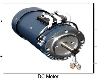
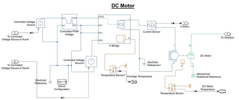
DC Motor:

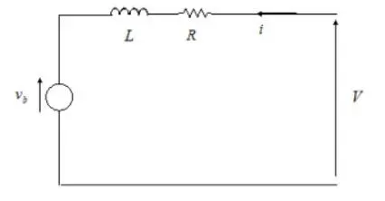
The DC Motor block represents the electrical and torque characteristics of a DC motor using the following equivalent circuit model. Here in this model the positive terminal was connected to the current sensor negative terminal and negative terminal was connected to the negative terminal of the H-Bridge. Additionally, the temperature port which is normally absent in the default condition was turned ON (by right clicking on the block then Simscape -> Block Choices -> Show Thermal Port) to monitor the temperature rise of the motor when in use by the vehicle, thereafter the port H appears on the block where the temperature sensor with thermal reference was connected.

Here, R is the rotor shaft of the DC motor which is further connected to the rotor shaft of the gear box in the Vehicle body subsystem and C is the DC motor Case which is connected to the mechanical rotational reference. The configured parameters considered for the DC motor in this model is as shown below.

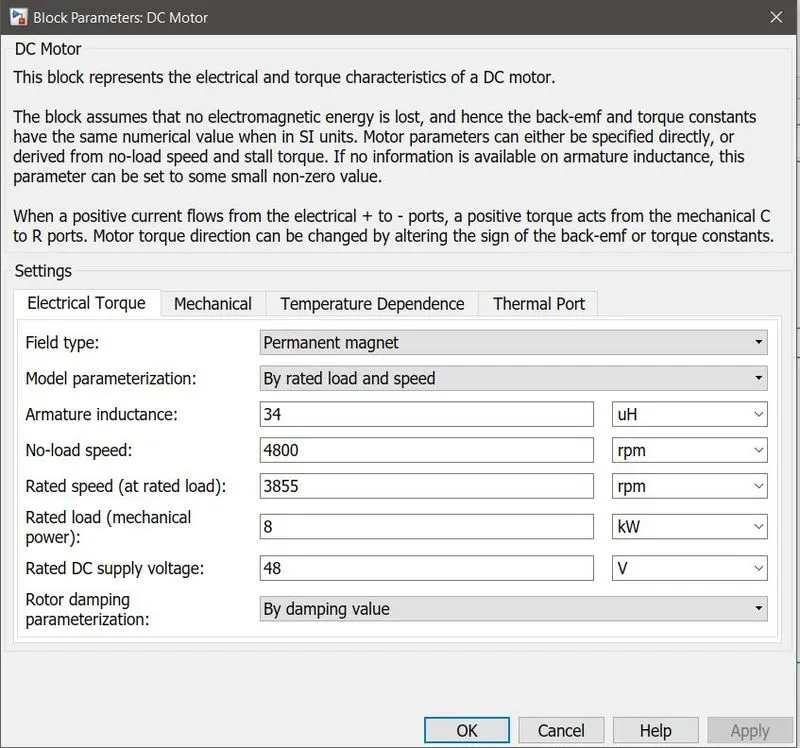
Mechanical Properties:

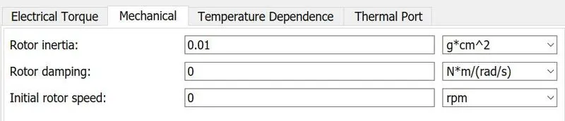
Temperature Dependence:

Thermal Port:

For this model the no-load speed was set to 4800 rpm, which is the speed of the motor when not driving a load and the rated speed was set to 3855 rpm, which is the motor speed at rated mechanical power level.

Temperature Sensor:

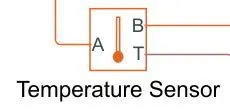
This block measures temperature in a thermal network. There is no heat flow through the sensor. The physical signal port T reports the temperature difference across the sensor. The measurement is positive when the temperature at port A is greater than the temperature at port B.

Thermal Reference:

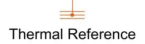
This block represents a reference point in a thermal network where the temperature is equal to absolute zero.

Mechanical Rotational Reference:

This block represents a mechanical rotational reference point, that is, a frame or a ground.

H-Bridge:

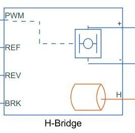
Block parameters:

Input Thresholds:

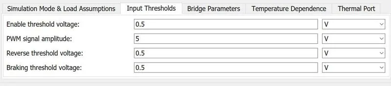
Enable threshold voltage: 0.5 V, this is voltage above value of PWM at which the H-Bridge starts.

PWM signal amplitude: 5.0 V, it is the amplitude of the signal at the PWM input, which was kept as a default value.

Reverse threshold voltage: 0.5 V

Braking threshold voltage: 0.5 V

Bridge Parameters:

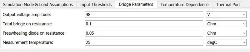
Output voltage amplitude: 48 V, this is the parameter that will be active only when “Internal” is selected for power supply mode of the H-Bridge and this is an amplitude of the voltage across the H-Bridge.

Total bridge on resistance: 0.1 Ohm

Freewheeling diode on resistance: 0.05 Ohm, default values were kept as same.

Measurement temperature: 25 degC

Temperature Dependence:

Thermal Port:

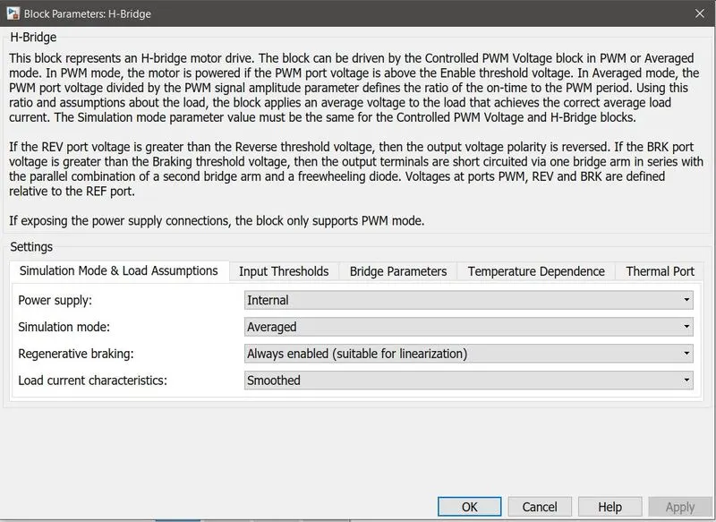
Simulation Mode and Load Assumptions:

Power Supply: The power supply was selected to the Internal mode which is default.

Simulation mode: Averaged was selected as the time take to simulate in Averaged mode is less compared to when selected PWM mode. When selected Averaged mode this has two options: Regenerative Braking and Load current characteristics.

Regenerative Braking: was selected to be always enabled as regenerative braking is very useful to generate vehicle’s own electricity when braking or decelerating.

Load Current characteristics: Smoothed was the default option as it assumes that the current is practically continuous due to load inductance.

H-Bridge Connection Ports:

PWM: Pulse width modulus signal, in this the controlled PWM voltage block output port “PWM” is connected to this port.

REF: This is the reference port which is an electric conversing port associated with floating zero volts.

REV: Reverse port.

BRK: Brake port.

In this block, the PWM port is connected to the PWM port of the controlled PWM voltage block, REF and REV are connected to the REF block of the controlled PWM voltage block. The BRK port is connected to the another controlled voltage source which has input from the DecelCmd of the Longitudinal Driver. The positive terminal of H-Bridge is connected to the positive port of the current sensor and further connected to the positive terminal of the DC motor via negative terminal of the current sensor and the negative terminal is connected to the negative terminal of the DC motor.

H: Temperature Sensor port where temperature sensor was connected with the thermal reference block as explained earlier.

Current Sensor:

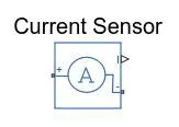
This block represents an ideal current sensor, that is, a device that converts current measured in any electrical branch into a physical signal proportional to the current. Connections + and - are conserving electrical ports through which the sensor is inserted into the circuit. Connection I is a physical signal port that outputs current value. Here the positive terminal is connected to the positive of H-Bridge and the negative terminal is connected to DC motor positive terminal, terminal I is connected to the battery subsystem for the current output monitoring via PS-Simulink converter.

Controlled PWM Voltage:

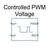
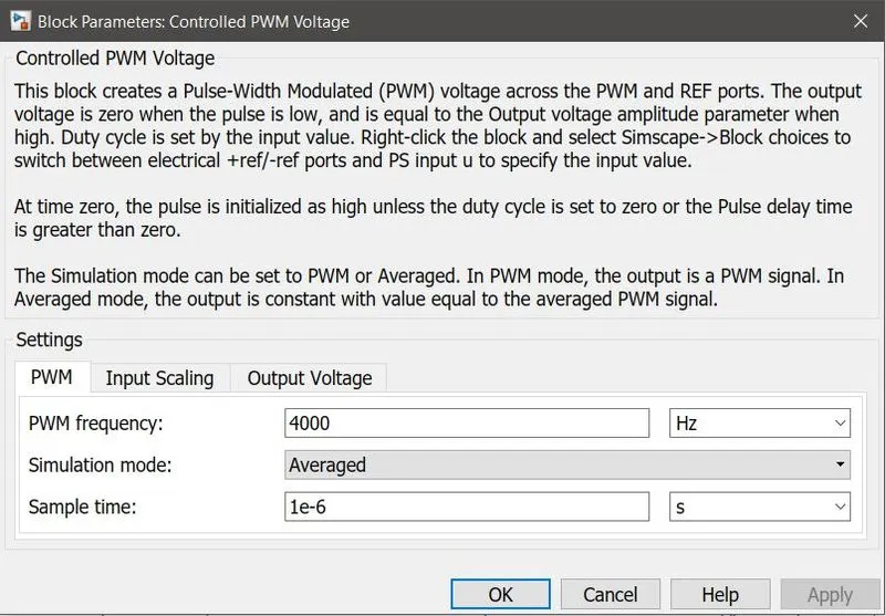
This block creates a Pulse-Width Modulated (PWM) voltage across the PWM and REF ports. The output voltage is zero when the pulse is low and is equal to the Output voltage amplitude parameter when high.

The block parameters were kept default for this block.

Port Connections:

ref+: Positive terminal, it is the positive electrical reference terminal connected with the controlled voltage source’s positive terminal which receives the drive cycle inputs from the AccelCmd port of the Longitudinal Driver.

ref-: Negative terminal, connected to the electrical reference (ground) and the negative terminal of controlled voltage source.

PWM: Pulse width modulated signal; an electrical reference signal port connected to the PWM port of the H-Bridge ­

REF: Floating zero reference, connected to REF and REV ports of the H-Bridge.

Controlled Voltage Source:

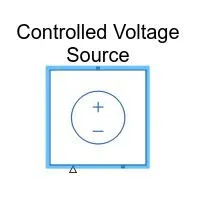
The block represents an ideal voltage source that is powerful enough to maintain the specified voltage at its output regardless of the current passing through it. This block has one physical signal input port and two electrical ports associated with its electrical terminals.

Two of these blocks were used in this subsystem one for acceleration command coming from the longitudinal driver and one for the deceleration command coming from the longitudinal driver.

Solver Configuration:

This block is needed to start the simulation and is used in solving the Simulink model. This block is connected to the controlled PWM voltage and H-Bridge blocks with the electrical reference (ground).

Vehicle Body Subsystem:

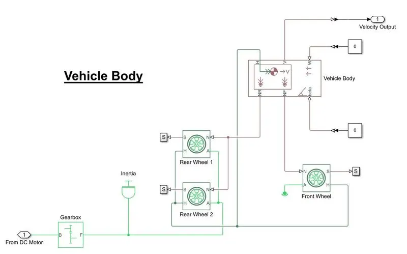
Vehicle Body Block:

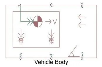
Vehicle Body block represents a two-axle vehicle body in longitudinal motion. The block accounts for body mass, aerodynamic drag, road incline, and weight distribution between axles due to acceleration and road profile. The vehicle can have the same or a different number of wheels on each axle. Optionally include pitch and suspension dynamics or additional variable mass and inertia. The vehicle does not move vertically relative to the ground.

Input and Output Terminals of the block:

• W: Physical signal input port for headwind speed.
• beta: Physical signal input port for road incline angle.
• H: Conserving port associated with the horizontal motion of the vehicle body. Connect tire traction motion to this port.
• NR: Physical signal output port for normal force on the rear axle. Wheel forces are considered positive if acting downwards.
• NF: Physical signal output port for normal force on the front axle. Wheel forces are considered positive if acting downwards.
• V: Physical signal output port for vehicle longitudinal velocity.

The vehicle body parameters were changed from the default values which can be seen below.

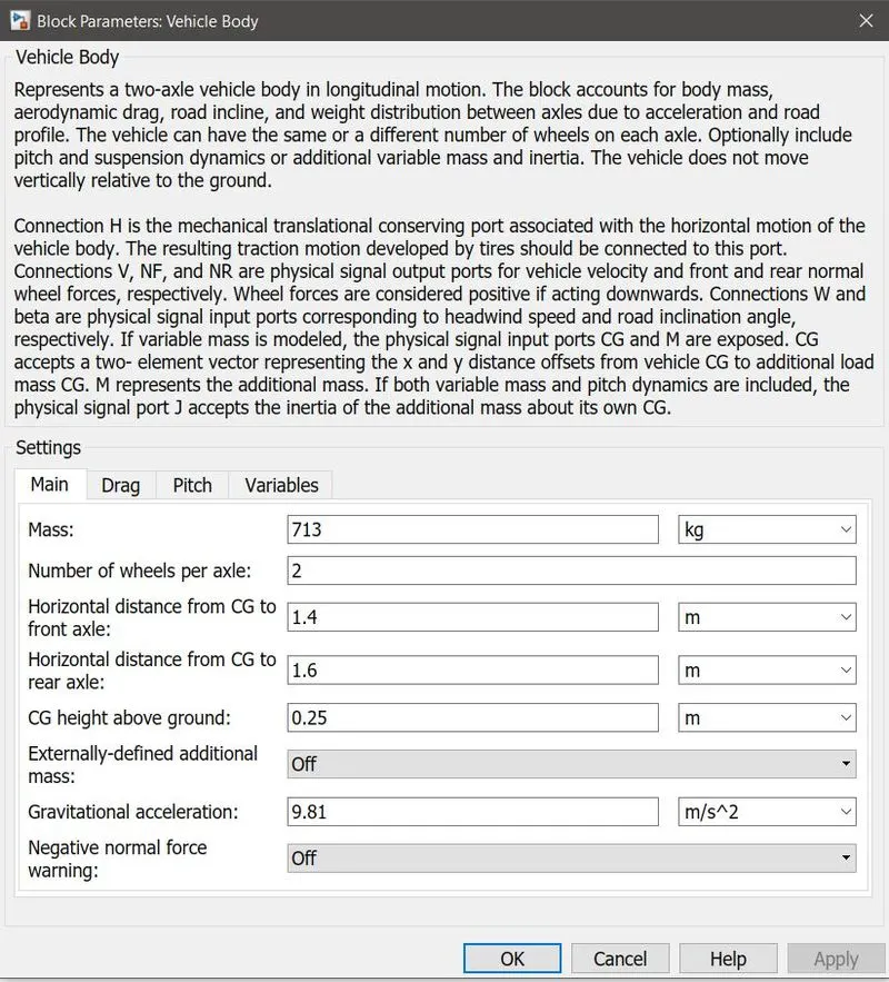
Parameters:

• Main parameters:
  1. Mass: 600kg
  2. Number of wheels per axle: 2
  3. Horizontal distance from CG to front axle:4m
  4. Horizontal distance from CG to rear axle:6m
  5. CG height above ground:25m
  6. Externally-defined additional mass: off
  7. Gravitational acceleration:81m/s^2
  8. Negative normal force warning: off
• Drag parameters:
  1. Frontal area: 48m^2
  2. Drag coefficient:5
  3. Air density:81kg/m^3
• Pitch:
  1. Pitch dynamics: off
• Variables:
  1. Beginning value of Velocity: 0

The inputs for wind velocity (W) and incline angle (beta) were not considered for the simulation therefore were connected to a constant block with zero value.

Tire (magic formula):

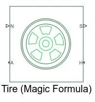
The Tire (Magic Formula) block models the tire as a rigid wheel-tire combination in contact with the road and subject to slip. When torque is applied to the wheel axle, the tire pushes on the ground (while subject to contact friction) and transfers the resulting reaction as a force back on the wheel. This action pushes the wheel forward or backward. If you include the optional tire compliance, the tire also flexibly deforms under load.

The figure shows the forces acting on the tire. The table defines the tire model variables.

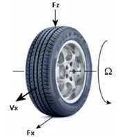
Where,

• Fz: Vertical load on tire
• Fx: Longitudinal force exerted on the tire at the contact point
• Vx: Wheel hub longitudinal velocity
• Ω: Wheel angular velocity

Block Terminals:

• N (Normal Force): Physical signal input port associated with the normal force acting on the tire. The normal force is positive if it acts downward on the tire, pressing it against the pavement.
• S (Slip): Physical signal output port associated with the relative slip between the tire and road.
• H (Hub): Mechanical translational port associated with the wheel hub that transmits the thrust generated by the tire to the remainder of the vehicle.
• A (Axle): Mechanical rotational port associated with the axle that the tire sits on. This port is connected to the simple gear transmission.

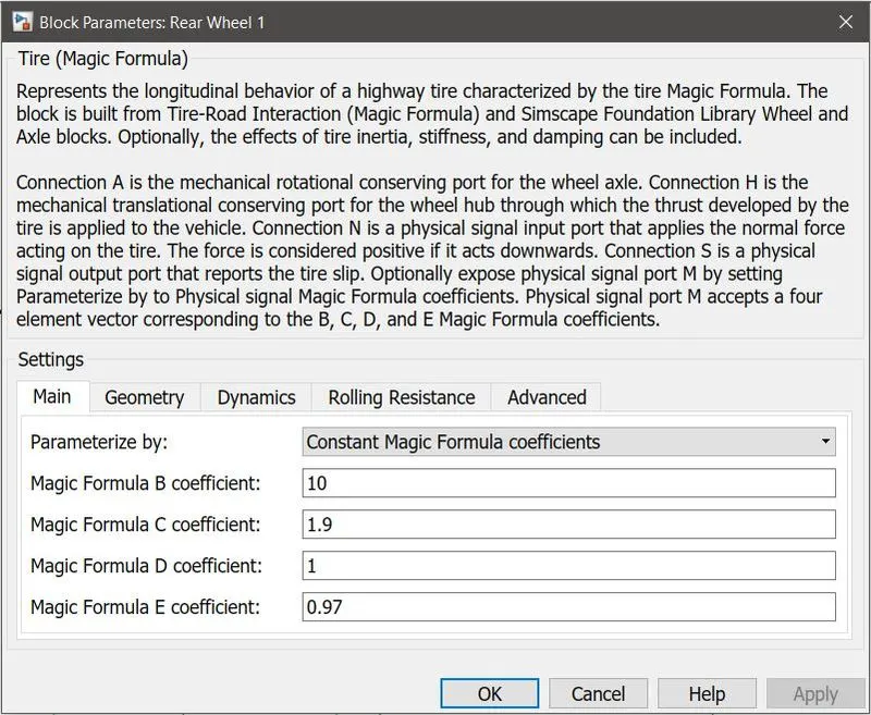
The block parameters are as shown below. The option Parameterize by was changed to Constant Magic formula coefficients and default values were considered for the model.

Geometry:

The parameters were kept same for all four wheels.

Inertia Block:

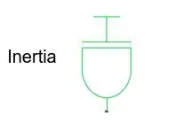
The block represents an ideal mechanical rotational inertia.

The block has one mechanical rotational conserving port. The block positive direction is from its port to the reference point. This means that the inertia torque is positive if the inertia is accelerated in the positive direction.

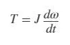
Where,

• T: Inertia torque
• J: Inertia
• ω: Angular velocity
• t: Time

Block Parameters:

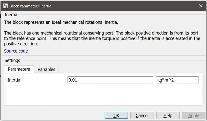
Here the inertia is kept at 0.01 kg*m^2 at default value. This block is connected to the rear axle of the vehicle body and the simple gear as axle and gear shaft are rotating parts.

Simple Gear Block:

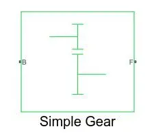
The Simple Gear block represents a gearbox that constrains the connected driveline axes of the base gear, B, and the follower gear, F, to co-rotate with a fixed ratio that you specify. You choose whether the follower axis rotates in the same or opposite direction as the base axis.

Simple Gear block parameters:

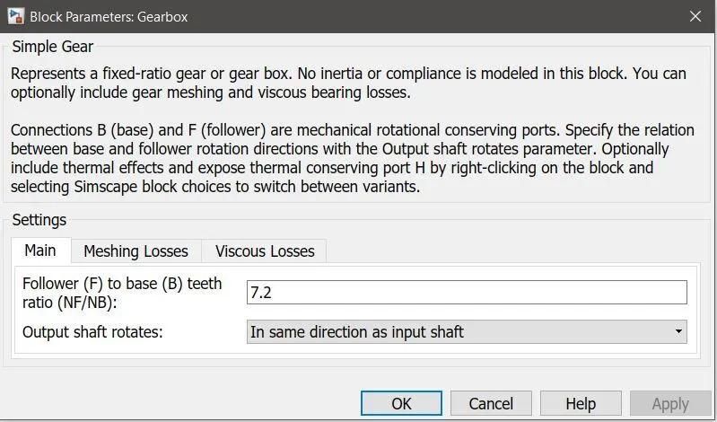
• Main:

1. Follower (F) to base (B) teeth ratio (NF/NB): 7.2
2. Output shaft rotates: In same direction as input shaft.

• Meshing Losses:

1. Friction model: No meshing loss – Suitable for HIL Simulation

The full electric model description completes here and the results and outcomes are discussed further on.

Results:

FTP75 DRIVE CYCLE:

After running the model for 2474 secs, total distance found out to be,

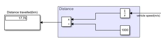
Below  graph shows the battery usage of vehicle for travelling 17.76km in 2474sec. And it is found to be approx 78% still left. And on the other graph current output is shown, it is quite fluctuating as speed input is so.

Below graph shows the input vs output speed comparison graph. And we could see that output speed is very much similar to input but could not overlap it during acceleration and sudden deacceleration.

WOT:

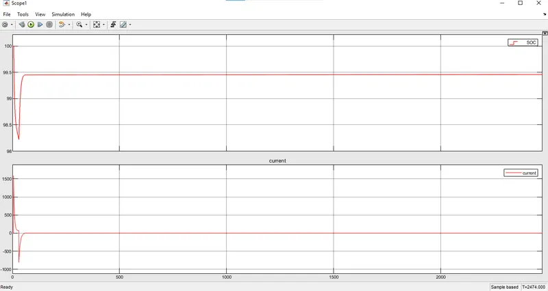
Ater running the model for 60secs the distance travelled is 0.477km.

The graph below shows the usage of battery and current output. In battery we can see regenerative battery technique is also been seen clearly. 

The graph below shows the input vs out output graph for speed. Here we can see that no matching in both the conditions is seen, this is due to short time running of vehicle. 

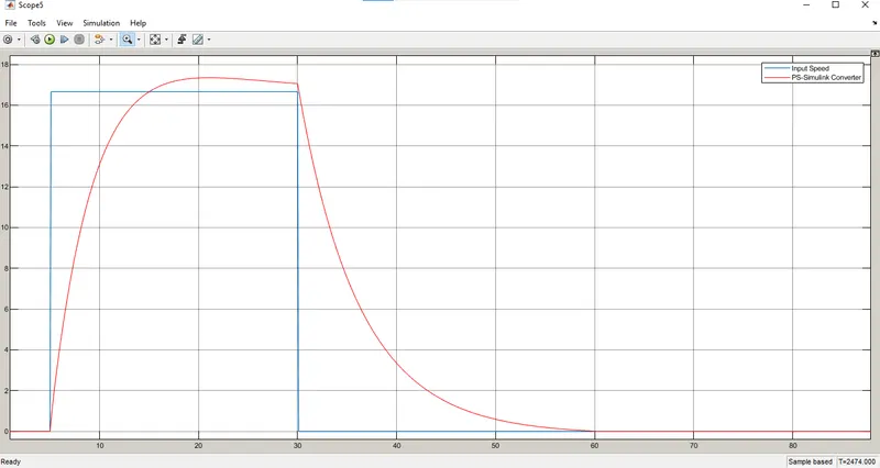
Signal builder input:-

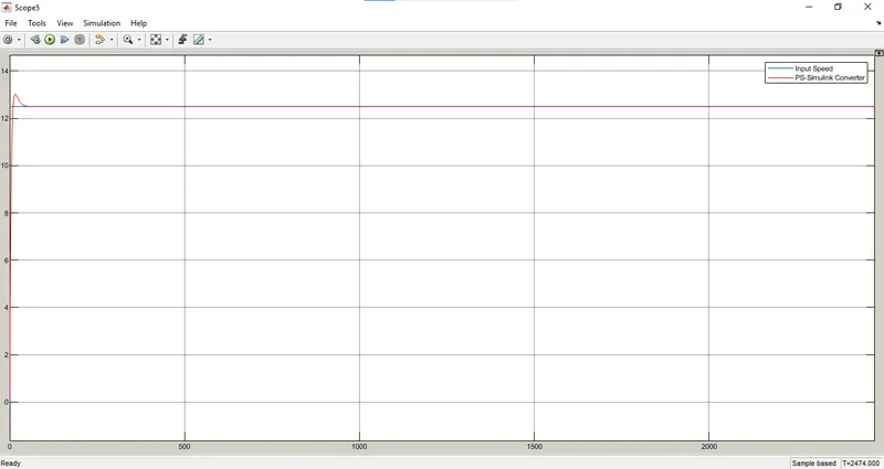
The graph below shows the output of the given signal builder which was for continuous 45kmph for 100km.

It shows the input signal and practical output as graph. We can see that its overlapping but the distance covered will not be exactly same as compared to input.

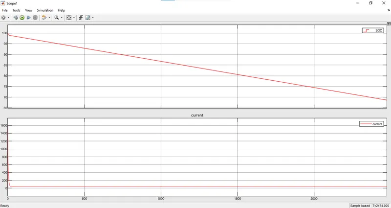
 The graph below shoes the battery % drop to travel 100km at 45kmph. It is still 65-68% left. And on th other graph current applied is shown.

The figure below shows the rise in temperature of controller while travelling given distance and comes to be approx 286degree c.

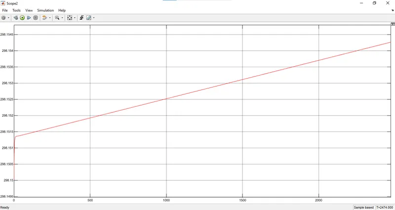
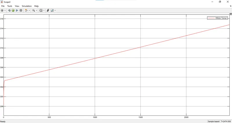
The figure below shows the graph of rise in temperature of motor with rise in speed na dtime. And it comes out to approx 315degree c.

 CONCLUSION:-

In this project we made a detailed model of electric rickshaw with proper modeling and 3 types of input is been provided for better understanding of input/output results.