Final Project: Electric Rickshaw modelling

Electric Rickshaw modelling.

Create a detailed MATLAB model of an electric rickshaw (three wheel passenger vehicle) as per details below:

Rear wheels driven by PM brushed type motor

Assume efficiency points of motor controller and motor

Make an excel sheet of all input and assumed data

Results: For any three standard driving cycles show energy consumption, temperature rise of motor and controller for 100 km constant speed driving at 45 kmph.

(Note- The simulink model file should be compulsorily attached)

Electric Rickshaws are eco-friendly battery-operated three-wheelers that have a better economy and lower operational cum maintenance costs. These e-rickshaws does not emit toxic pollutants into the air during operation and hence, does not have any tailpipe. These vehicles have gained popularity amongst Indian rickshaw drivers and commuters.

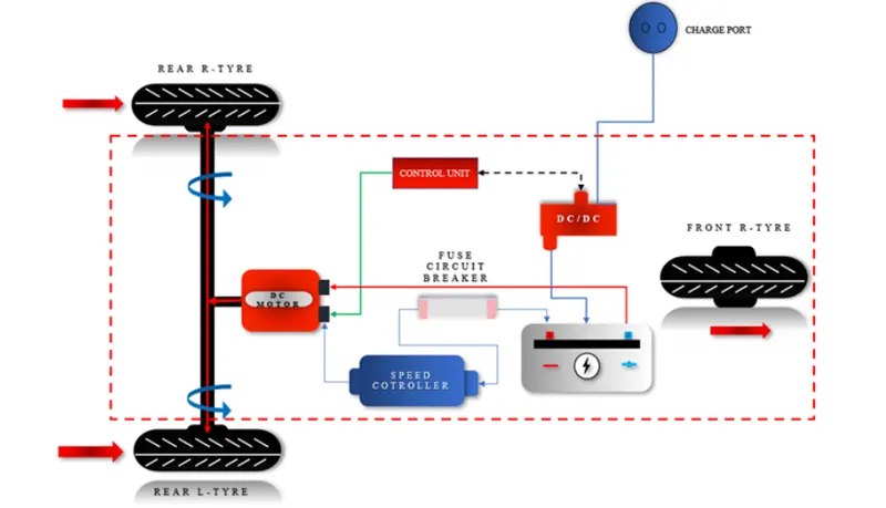
It consists of a controller unit.They are sold on the basis of voltage supplied and current output, also the number of mosfet (metal oxide field effect transistors) used. The vehicle's batteries are typically lead acid with a lifespan of 6–12 months. Deep cycle batteries designed for electric vehicles are rarely used. Weight of the electric car has also been a recurring design difficulty in them.

The chassis is the main part which ensures drive quality and safety of the vehicle. It is made of mild steel. These days, most of the locally-made chassis are often built without proper design, leading to an imbalance in the drive, and often causing the vehicle to pivot or topple very easily. The chassis manufactured by a professional E Rickshaw Manufacturer is robust as the design adheres to all quality / technical parameters, which are often ignored by others. The chassis, if inaccurately mad

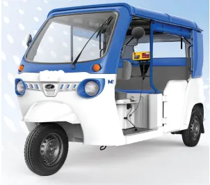
Genaral deatils of the E-Rickshaw:

1) Battery type: lithium-ion 330v75

2) vehicle kerb weight 260 kgs

3) load capacity 340 kgs

4) vehicle speed 7kmph

5) driving range 140 km (160ah)

6)no of wheels per axel 2

7)frontal area 91 m

8) drag coefficeient 5 wheel radius 306m

9) vertical load 3000N

10) nominal volatge 330v

11) rated capacity 75Ah

12) initial SOC 100%

13) internal resistance 5ohms

Procedure:-

Main Subsystem of the Electric-vehicle.

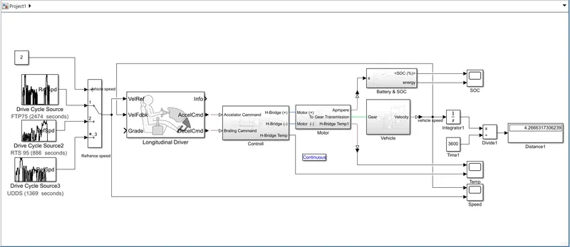
For modelling the whole vehicle in SIMULINK. we need to model the above emntioned components separately and make them work together.

All the main components are available in the library of SIMULINK blocks.

so we add components and configure the parameters to fit the the working requirements of the model.

In This We Implement the Five SubSystems.

1. Vehicle.
2. Motor.
3. Controller.
4. Battery and State Of Charge.(SOC)
5. Longitudinal Drive Block.
6. Drive Cycle.

1. Subsystem Of the Vehicle.

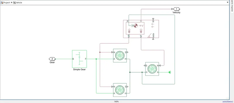
In This Subsystem Consist Of Following Componants Or Parts:-

1. Tire:-

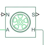
1. H is noting but HUB.
2. A is nothing but the axel.
3. N is the normal force.
4. S stands for slip.

• We selected The Three Tire For auto Rikshaw we consider Left of the Two tire as a rear tire and N Port of the tire conected to NR port of the vehicle body.
• And we consider Right of the tire as a front tire and N Port of the tire conected to NF port of the vehicle body.
• H port of the Tire is conected to the H port of the vehicle body.
• Left of the Axel Port (A) is going to the Gear System Of the F port.

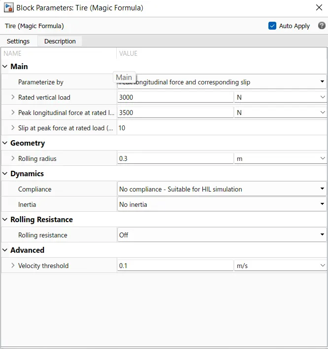
Parameters Of The Block.

2. Vehicle Body :-

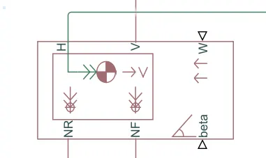
• Represents a two-axle vehicle body in longitudinal motion. The block accounts for body mass, aerodynamic drag, road incline, and weight distribution between axles due to acceleration and road profile.
• The vehicle can have the same or a different number of wheels on each axle. Optionally include pitch and suspension dynamics or additional variable mass and inertia.
• The vehicle does not move vertically relative to the ground.
  Connection H is the mechanical translational conserving port associated with the horizontal motion of the vehicle body. The resulting traction motion developed by tires should be connected to this port.
• Connections V, NF, and NR are physical signal output ports for vehicle velocity and front and rear normal wheel forces, respectively. Wheel forces are considered positive if acting downwards.
• Connections W and beta are physical signal input ports corresponding to headwind speed and road inclination angle, respectively.
• If variable mass is modeled, the physical signal input ports CG and M are exposed. CG accepts a two- element vector representing the x and y distance offsets from vehicle CG to additional load mass CG.
• M represents the additional mass. If both variable mass and pitch dynamics are included, the physical signal port J accepts the inertia of the additional mass about its own CG

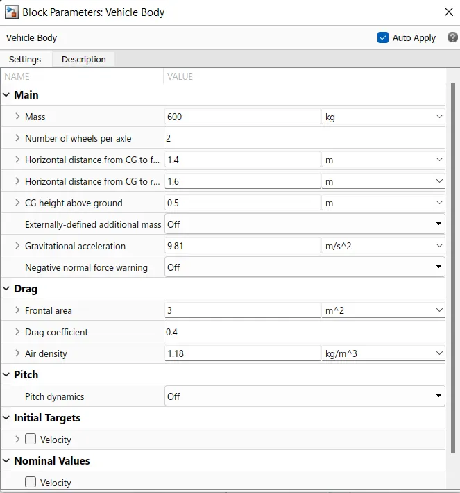
Parameters Of The Block.

3. Gear System.

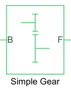
• Represents a fixed-ratio gear or gear box. No inertia or compliance is modeled in this block. You can optionally include gear meshing, backlash, and viscous bearing losses.
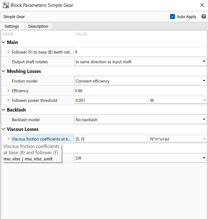
• Connections B (base) and F (follower) are mechanical rotational conserving ports. Specify the relation between base and follower rotation directions with the Output shaft rotates parameter.
• Optionally include thermal effects and expose thermal conserving port H by setting Friction model to a temperature-dependent setting.

Parameters Of The Block.

4. Rotational Free End.

This block represents a mechanical rotational free end. Use it to allow a node to rotate freely without torque. This block can be used to optionally specify initial rotational velocity.

2. Sub-system Of the Motor.

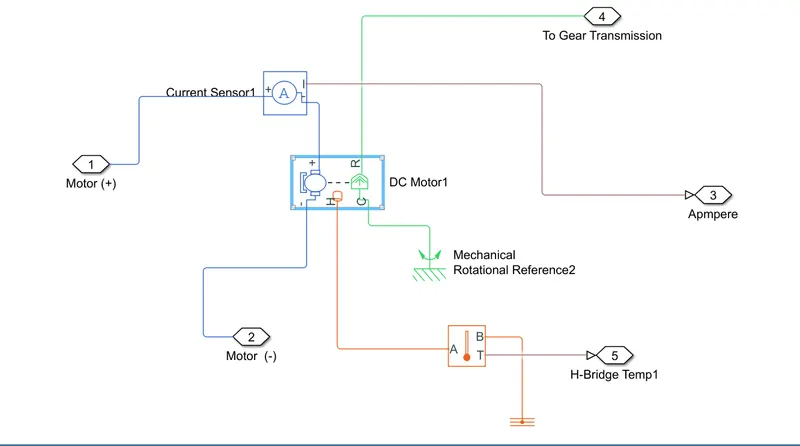
In This Subsystem Consist Of Following Componants Or Parts:-

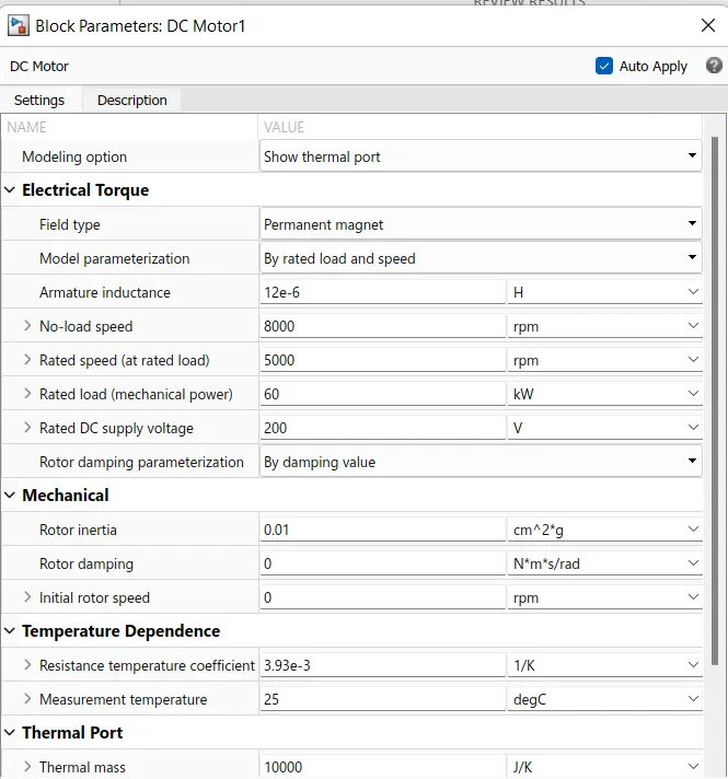
1. DC Motor:-

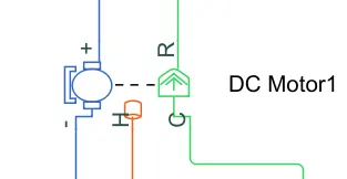
• For EV model we selected the DC motor block Which Is Permanant Magnet Brush Type DC Motor And implementation is simle compare to others and its have few parameters.
• In This motor Block two sides which is Right one is mechanical side and Left is electrical side.
• In mechanical side has a two ports C And R. C is the nothing but the casing and it is standstill And R is nothing But the Rotor Which is produced the toque.
• In electrical side Two Ports Which Possitive and anather is Negative for voltage is applied. the possitive port is going to the possitive side of the H-bridge through the current sensor block and negative is connected to the Negative side of the H-Bridge.
• Mechanical side R port is connected to the gear in the vehicle body block And C port is connected to the Rotational Reference Block because the its stationary.
• In this H-Port is Connect to Temprature Sensors.

Parameters Of The Block.

2. Current Sensor :-

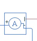
• This device that converts current measured in any electrical branch into a physical signal proportional to the current.
• In this Two Port + and - are conserving electrical ports through which the sensor is inserted into the circuit. Connection I is a physical signal port that outputs current value.

3. Temprature Sensor :-

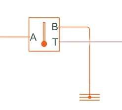
This block measures temperature in a thermal network. There is no heat flow through the sensor. The physical signal port T reports the temperature difference across the sensor. The measurement is positive when the temperature at port A is greater than the temperature at port B.

4. Mechanical Rotational Refrance :-

This block represents a mechanical rotational reference point, that is, a frame or a ground. Use it to connect mechanical rotational ports that are rigidly affixed to the frame (ground).

3. Sub-system Of the Controller.

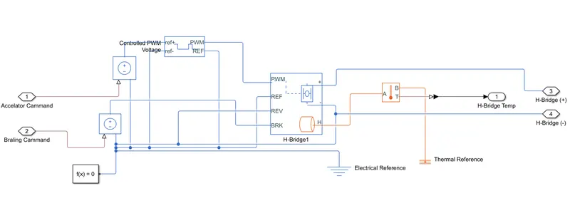
In This Subsystem Consist Of Following Componants Or Parts:-

1. H-Bridge:-

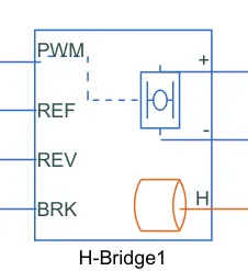
• This is a power converter which is needed to provide power of the correct form and magnitude from one component to other.
• In case of EV,s a power converter is needed to provide a DC voltage from the battery of the EV to the DC motor, so that it can fuction properly at the required parameters.
• Here i have used an H-bridge motor drive as my power converter.
• The left side is for controlling the voltage signalsand the right side terminals to provide the controlled voltage to the DC motor the left side ports are:

1. PWM- Pulse width modulation
2. REF- Reference
3. REV- Reverse
4. BRL- Brake
5. H-Temp.

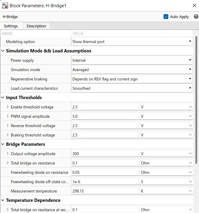
Parameters Of The Block.

2. Controlled PWM Voltage Block.

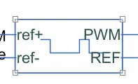
• This block creates a Pulse-Width Modulated (PWM) voltage across the PWM and REF ports.
• The output voltage is zero when the pulse is low, and is equal to the Output voltage amplitude parameter when high.
• Duty cycle is set by the input value.
• At time zero, the pulse is initialized as high unless the duty cycle is set to zero or the Pulse delay time is greater than zero.
• The Simulation mode can be set to PWM or Averaged. In PWM mode, the output is a PWM signal. In Averaged mode, the output is constant with value equal to the averaged PWM signal.

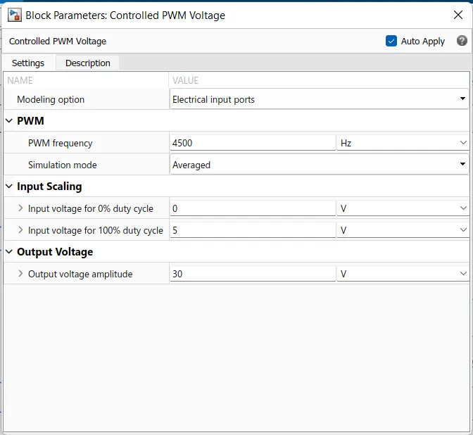
Parameters Of The Block.

3. Controlled Voltage Source.

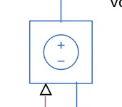
• The block represents an ideal voltage source that is powerful enough to maintain the specified voltage at its output regardless of the current passing through it.
• The output voltage is V = Vs, where Vs is the numerical value presented at the physical signal port.

4. Solver Configuration.

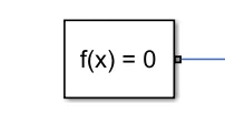
Defines solver settings to use for simulation.

4. Electrical Refrance.

Electrical reference port. A model must contain at least one electrical reference port (electrical ground).

4.Subsystem of Battery and State Of Charge.(SOC)

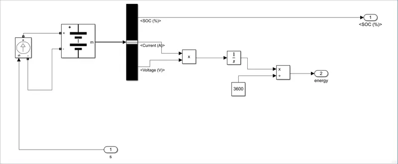
In This Subsystem Consist Of Following Componants Or Parts:-

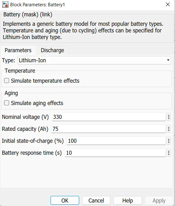
1. Battery.

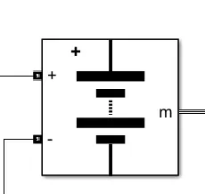
• We Select the Lithium-Ion battery type.
• Nominal Voltage is 330 V for our condition and Internal Resistance is 0.2 ohm.

Parameters Of The Block.

2. Controlled Current Source.

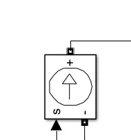
• The block represents an ideal current source that is powerful enough to maintain the specified current through it regardless of the voltage across it.
• The output current is I = Is, where Is is the numerical value presented at the physical signal port.

3. Integrator.

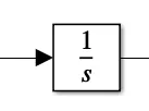
Continuous-time integration of the input signal.

5. Longitudinal Driver Block.

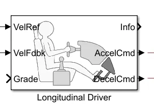
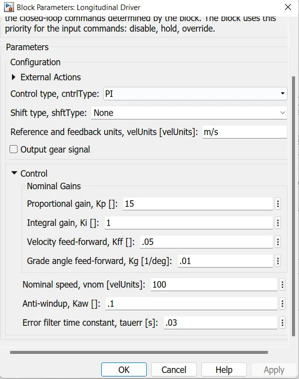
The longitudinal driver block is used for giving normalized acceleration and deacceleration commants to a controller based on two sets of data. The first data is the reference velocity and second data is the feedback velocity.The reference velocity data coming from drive cycle source and is compared to the feedback velocity data coming from the vehicle body. If the reference velocity is greater than the feedback velocity, an acceleration comand will be given as an output to the controlled voltage source. If the reference velocity is lesser than the feedback velocity, a deacceleration command is given as output to anpother controll voltage source. For the output acceleration and deacceleration commands i have used simulink-PS converter block. In this case the input signal; is velocity data and this is logic data which have to be converted to a voltage signal The ports in this block are:

• Velref- This stands for the reference velocity and it is the velocity data provided from a drive cycle source.
• Velfdbl- This stands for feedback velocity and it is coming from the vehicle's body velocity port
• Grade- This port provides a grade or inclination angle on which the vehicle is travelling in degrees.
• Info- This port is for the bus signals which consists of block calculations
• Accelcmd- This port provides the acceleration command to a controlled voltage source
• Deacclcmd- This port provides the deacceleration command to another voltage source.

Parameters Of The Block.

6. Drive cycle.

In This We have Used Three Types Of Drive Cycle

1. FTP75 (2474 Sec).
2. RTS95 (886 Sec).
3. UDDS (1369 Sec).

A drive cycle is a data set that contains velocity and time data for the purpose of modelling the motion of a vehicle. It is a plot of the vehicle velocity against the time and it is made to resembl typicall driving conditions that a consumer may experience themselves in. Drive cycles are used by various testing procedures such as mileage, pollution tests, and acceleration and top speed tests.There are three ways of implementing a drive cycle. One method is to create your own drive cycle with spreedsheet or excelsheet. Another method isuse a signal builder and create siganls according to the user and the method that we used is to implement industry standard drive cycles which are previosly used to test parameters of the vehicle.

1. FTP75 (2474 Sec).

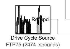
We Run the above drive cycle for We implimentd EV model and Take the outputs. The distance travelled by the vehicle in the drive cycle is also measured using the display block. Before simulation the run time was updated according to the drive cycle time 2474secs.

Scope Outputs As following.

1. Speed
2. State Of charge (SOC).
3. Temprature.

1. Speed.

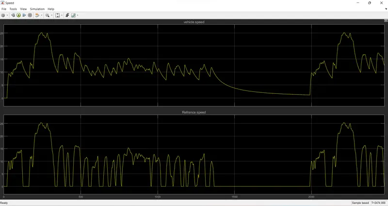
• From this scope we can see two signals. The Lower signal Shows the Drive Cycle Data and Upper Signal show the Implimented EV module which similer to Drive cycle Signal.
• As we can see that the longitudinal driver successfully maintains the drive cycle data , process it and controls the vehicle's speed according to the reference speed.
• the graph overlaps eachother effectively during acceleration and deacceleration.

2.State Of Charge(SOC).

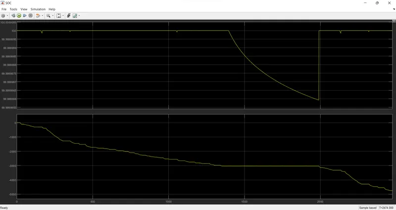
The SOC scope shows how the Two Graph Upper Graph Shwos the Energy And Lower Graph is Shwos the SOC

state of the battery varies over the drive cycle time, The batter was modelled to begin with an SOC pf 1 that is 100%. As the simulation starts the charge of the bettery gets decreased and when the vehicle is in braking mode the uplift in the grapf shows that regenerative braking is working to maintain the battery charge.

3. Temprature.

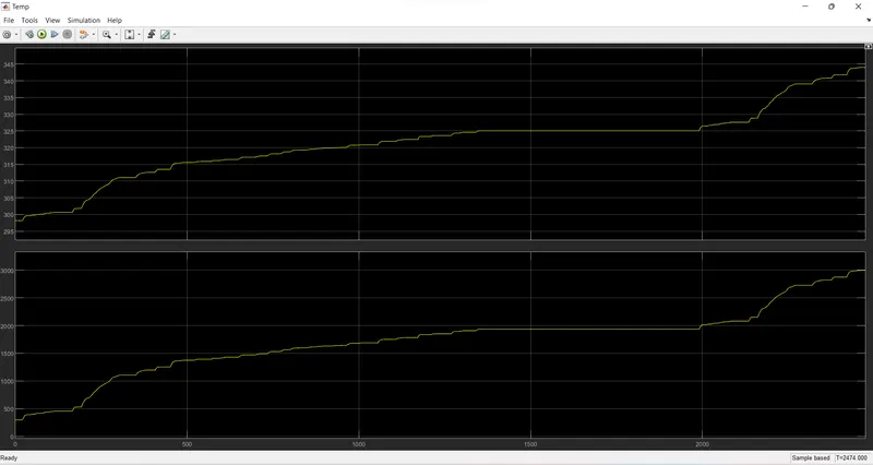
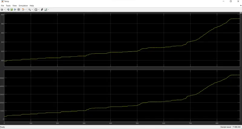
The temp Scope Shwos the Two Graph Upper Graph Is H-Bridge Temp and Lower Graph is Motor Temp.

4.Distance.

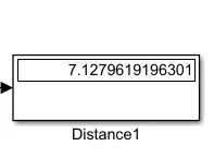
The Above Drive Cycle Verhicle Covered 7.12 Km Distance.

2. RTS95 (886 Sec).

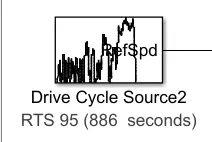
We Run the above drive cycle for We implimentd EV model and Take the outputs. The distance travelled by the vehicle in the drive cycle is also measured using the display block. Before simulation the run time was updated according to the drive cycle time 886secs.

1. Speed

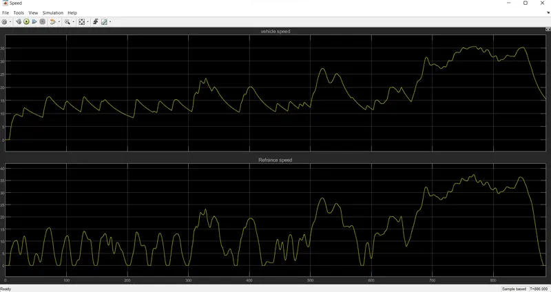
• From this scope we can see two signals. The Lower signal Shows the Drive Cycle Data and Upper Signal show the Implimented EV module which similer to Drive cycle Signal.
• As we can see that the longitudinal driver successfully maintains the drive cycle data , process it and controls the vehicle's speed according to the reference speed.
• the graph overlaps eachother effectively during acceleration and deacceleration.

2.State Of Charge(SOC).

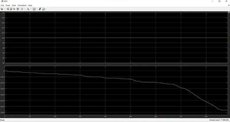
The SOC scope shows how the Two Graph Upper Graph Shwos the Energy And Lower Graph is Shwos the SOC

state of the battery varies over the drive cycle time, The batter was modelled to begin with an SOC pf 1 that is 100%. As the simulation starts the charge of the bettery gets decreased and when the vehicle is in braking mode the uplift in the grapf shows that regenerative braking is working to maintain the battery charge.

3. Temprature.

4. Distance.

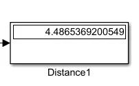
The Above Drive Cycle Verhicle Covered 4.48 Km Distance.

3. UDDS (1369 Sec).

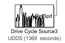
We Run the above drive cycle for We implimentd EV model and Take the outputs. The distance travelled by the vehicle in the drive cycle is also measured using the display block. Before simulation the run time was updated according to the drive cycle time 1369secs.

1. Speed.

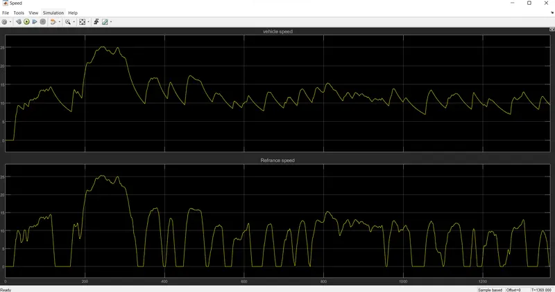
• From this scope we can see two signals. The Lower signal Shows the Drive Cycle Data and Upper Signal show the Implimented EV module which similer to Drive cycle Signal.
• As we can see that the longitudinal driver successfully maintains the drive cycle data , process it and controls the vehicle's speed according to the reference speed.
• the graph overlaps eachother effectively during acceleration and deacceleration.

2.State Of Charge(SOC).

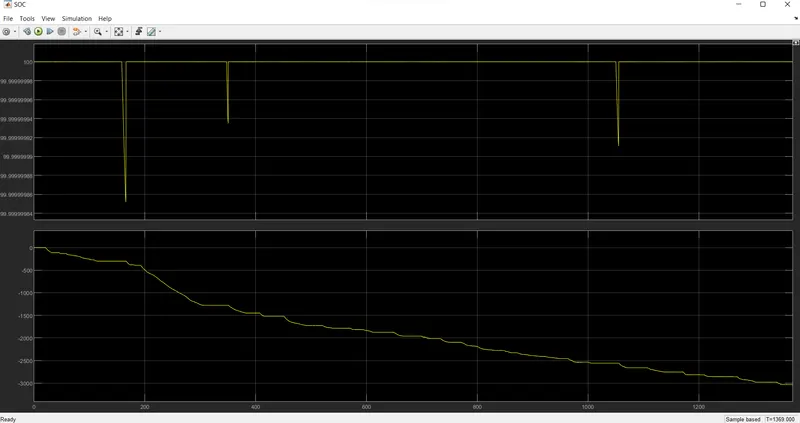
The SOC scope shows how the Two Graph Upper Graph Shwos the Energy And Lower Graph is Shwos the SOC

state of the battery varies over the drive cycle time, The batter was modelled to begin with an SOC pf 1 that is 100%. As the simulation starts the charge of the bettery gets decreased and when the vehicle is in braking mode the uplift in the grapf shows that regenerative braking is working to maintain the battery charge.

3. Temprature.

The temp Scope Shwos the Two Graph Upper Graph Is H-Bridge Temp and Lower Graph is Motor Temp.

4. Distance.

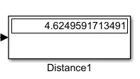
The Above Drive Cycle Verhicle Covered 4.62 Km Distance.