Final Project: Electric Rickshaw modelling
Create a detailed MATLAB model of an electric rickshaw (three wheel passenger vehicle).
Objectives:-
1] Rear wheels driven by PM brushed type motor.
2] Assume efficiency points of motor controller and motor.
3] Make an excel sheet of all input and assumed data.
4] Results:- For any three standard driving cycles show energy consumption, temperature rise of motor and controller for 100 km constant speed driving at 45 kmph.
Introduction:-
What is the Rikshaw?
A riksha or rickshaw is a kind of vehicle that has two or three wheels. They are usually pulled by a human but there are types that have been changed to be pulled by a bicycle or have their own motor. Then it is developed from rickshaw to Electric rickshaw using BLDC motor, Batteries.
The electric rickshaw also known as E-rickshaw have been becoming more popular in some cities since 2008 as an alternative to auto rickshaw and pulled rickshaw because of their low fuel cost, and less human effort compared to pulled rickshaw. They are being widely accepted as an alternative to petrol/diesel/CNG auto rickshaws.
The E-Rickshaw is a green solution with no petrol, CNG and mobile oil requirements. Electric rickshaw needs minimum maintenance and could serve as a solution to last mile commuting problems. They are 3 wheelers pulled by an electric motor (BLDC) and consists of differential mechanism at rear wheels. Basically these vehicles have a mild steel tubular chasis. THe elctrical system used in indian version is 48V DC can run 90-100 KM/full charge. The basic seating capacity of this rickshaw is 4+1.
Key Components of Electric Vehicles:-
Architecture of E-Rickshaw :-
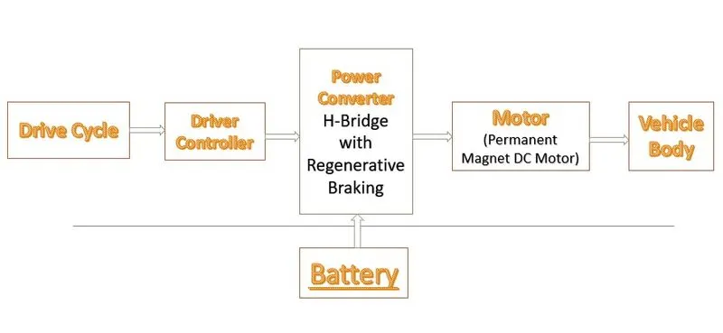
The simplest powertrain architecture consists in a 48 voltage battery, an electric motor with power electronics controller and a single speed gearbox. In this vehicle the propulsion is based exclusively on the electric energy stored in the battery.
Considering following data modelling the E-rickshaw in MATLAB/Simulink:-
Model of E-Rickshaw:-
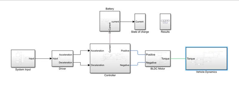
Description of this model:-
1] System Input Unit:-
For the control and input of whole model we give input which is 1] HWFET drive cycle, 2] Wide open throttle drive cycle 3] FTP 72 drive cycle.
For the selection inputs we used multiple switch. The inputs signal are passed through the corresponding to the truncated value of the first input. The inputs are numbered from top to bottom. The first input port is the control port. and other input ports are data ports.
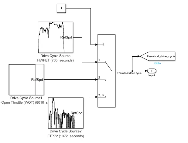
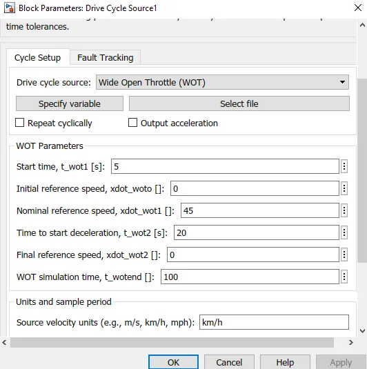
In WOT drive cycle we will calculate time as per given objective.
Time = Distance/speed = 100/(45/3600). since we want our drive cycle time in seconds so then converting kmph to kmps.
Time = 8000 seconds.
The drive cycle plot is shown below.
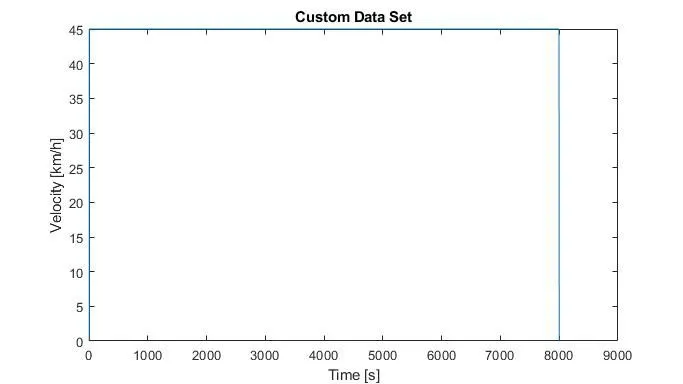
here it takes more time to simulate the model so i used this data
reference speed = 45kmph
deceleration = 20 seconds
simulation time = 100 seconds
2] Driver Unit:-
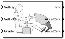
In this we use longitudinal driver block. In this the input is given actual velocity and Drive cycle and also given gradient then the driver give the output as acceleration and deceleration.
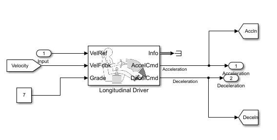
- Longitudinal Driver Block:-
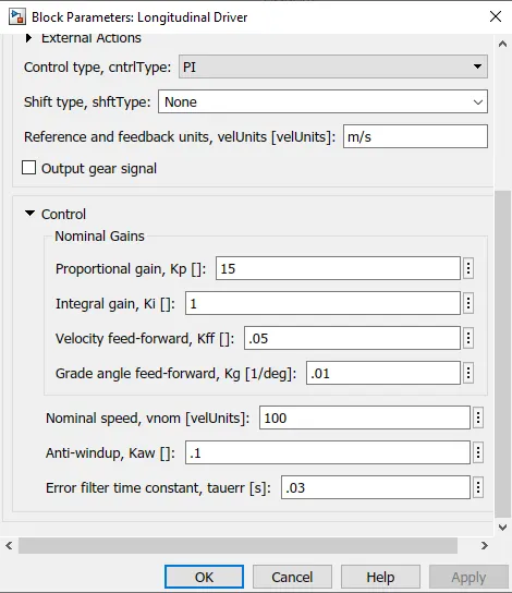
- Parameters:-
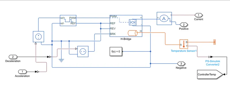
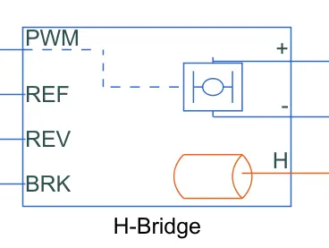
- H-Bridge Block:-
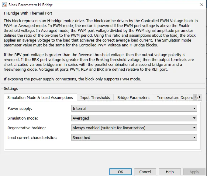
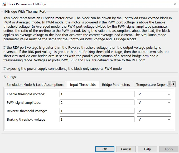
This block is used to change the polarity of the voltage applied across the DC motor so as to run the motor in forward and reverse direction as per the input command.
- Parameters:-
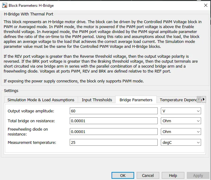
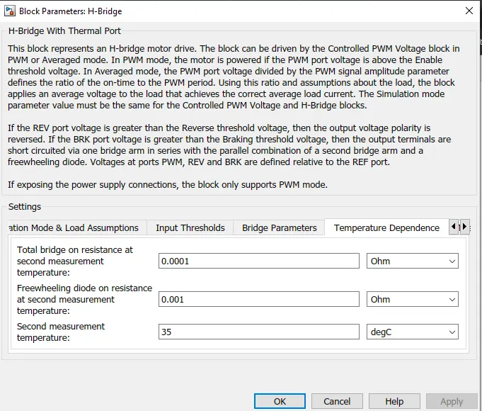
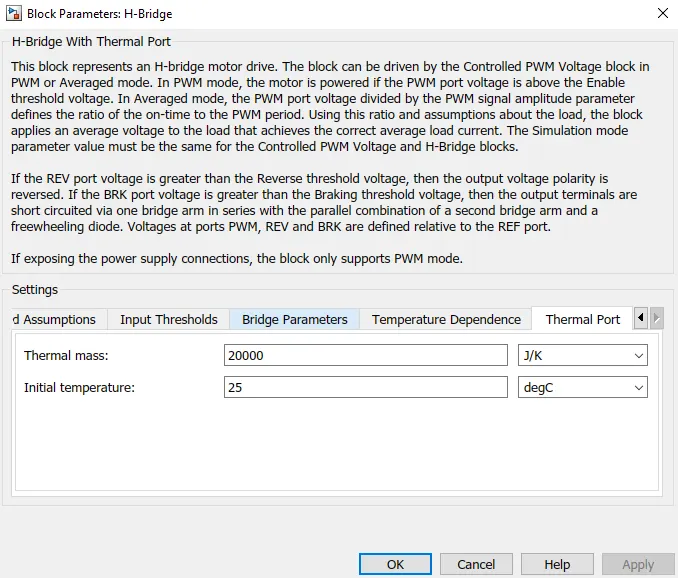
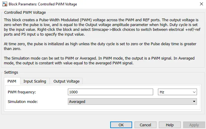
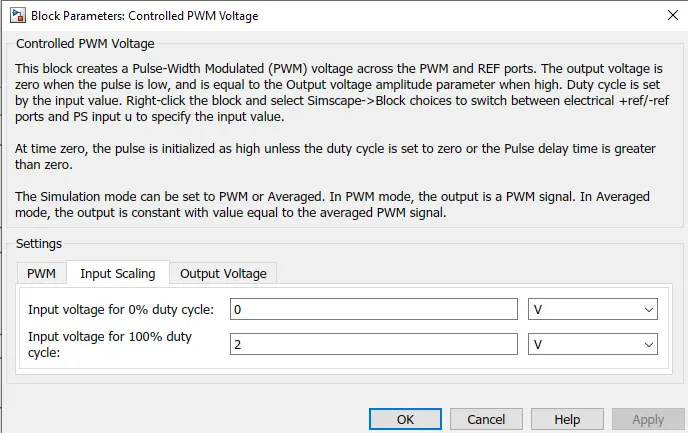
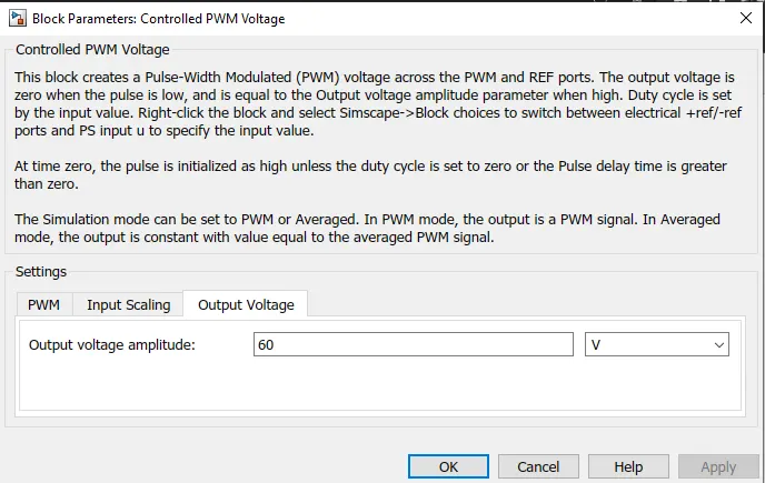
- Controlled PWM voltage block:-
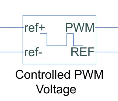
- Parameters:-
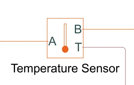
- Temperature Sensor Block:-
This block measures temperature in a thermal network. There is no heat flow through the sensor. The physical signal port T reports the temperature difference across the sensor. The measurement is positive when the temperature at port A is greater than the temperature at port B.
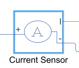
- Current Sensor Block:-
The block represents an ideal current sensor, that is, a device that converts current measured in any electrical branch into a physical signal proportional to the current.
Connections + and - are conserving electrical ports through which the sensor is inserted into the circuit. Connection I is a physical signal port that outputs current value.
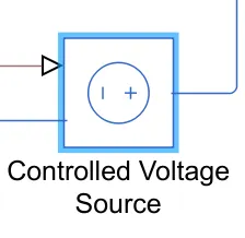
- Controlled Voltage Source Block:-
The block represents an ideal voltage source that is powerful enough to maintain the specified voltage at its output regardless of the current passing through it. The output voltage is V = Vs, where Vs is the numerical value presented at the physical signal port.
4] Permanent magnet brushed type motor Unit:-
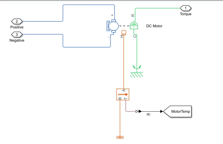
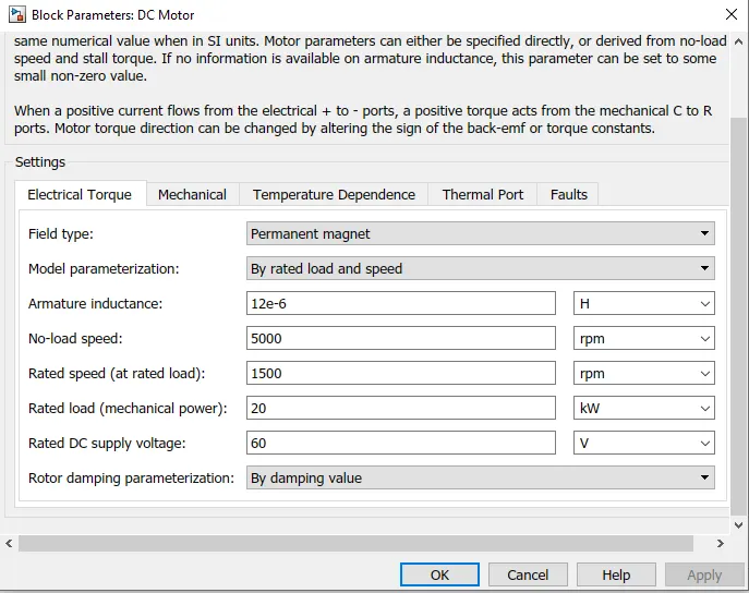
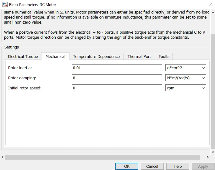
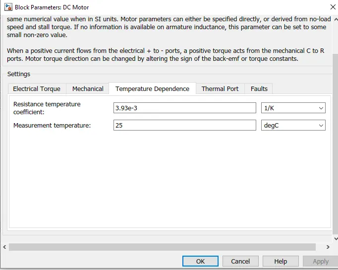
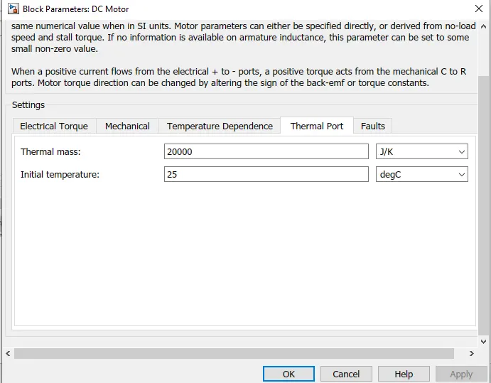
- DC motor with thermal port:-
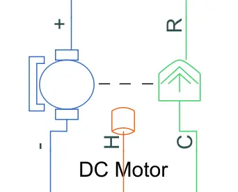
This block represents the electrical and torque characteristics of a DC motor.
The block assumes that no electromagnetic energy is lost, and hence the back-emf and torque constants have the same numerical value when in SI units. Motor parameters can either be specified directly, or derived from no-load speed and stall torque. If no information is available on armature inductance, this parameter can be set to some small non-zero value.
When a positive current flows from the electrical + to - ports, a positive torque acts from the mechanical C to R ports. Motor torque direction can be changed by altering the sign of the back-emf or torque constants.
- Parameters:-
5] Battery Unit:-
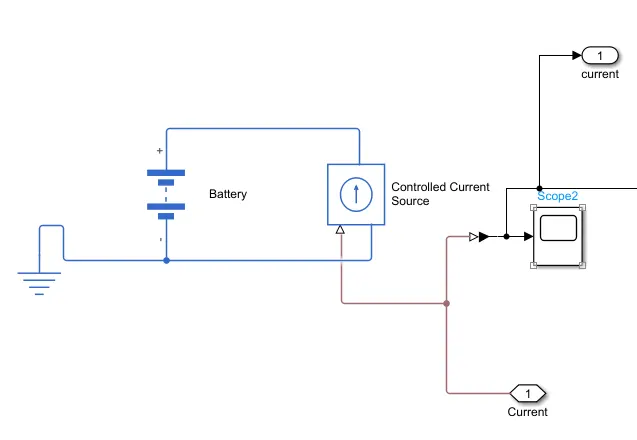
It is storage of electric power. from this the supply the power to all system of Rickshaw. When the DC current source will supplied from the battery then it is controlled and then send to system.
- Battery Block:-
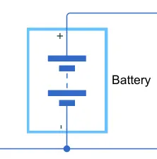
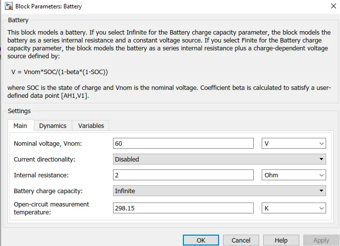
This block models a battery. If you select Infinite for the Battery charge capacity parameter, the block models the battery as a series internal resistance and a constant voltage source. If you select Finite for the Battery charge capacity parameter, the block models the battery as a series internal resistance plus a charge-dependent voltage source defined by:
V = Vnom*SOC/(1-beta*(1-SOC))
where SOC is the state of charge and Vnom is the nominal voltage. Coefficient beta is calculated to satisfy a user-defined data point [AH1,V1].
- Parameters:-
- Controlled Current Source Block:-
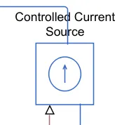
The block represents an ideal current source that is powerful enough to maintain the specified current through it regardless of the voltage across it. The output current is I = Is, where Is is the numerical value presented at the physical signal port.
6] Vehicle Dynamics Unit:-
This subsystem represents as a vehicle body and it is shown below.
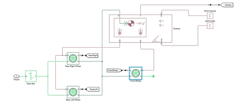
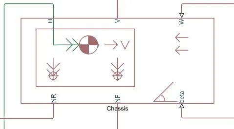
- Vehicle Body Block:-
Represents a two-axle vehicle body in longitudinal motion. The block accounts for body mass, aerodynamic drag, road incline, and weight distribution between axles due to acceleration and road profile. The vehicle can have the same or a different number of wheels on each axle. Optionally include pitch and suspension dynamics or additional variable mass and inertia. The vehicle does not move vertically relative to the ground.
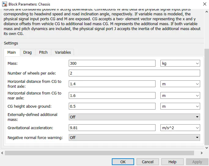
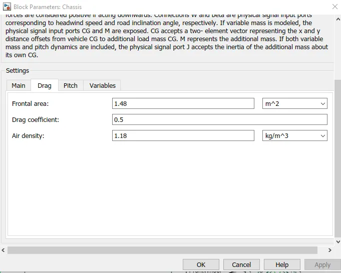
Connection H is the mechanical translational conserving port associated with the horizontal motion of the vehicle body. The resulting traction motion developed by tires should be connected to this port. Connections V, NF, and NR are physical signal output ports for vehicle velocity and front and rear normal wheel forces, respectively. Wheel forces are considered positive if acting downwards. Connections W and beta are physical signal input ports corresponding to headwind speed and road inclination angle, respectively. If variable mass is modeled, the physical signal input ports CG and M are exposed. CG accepts a two- element vector representing the x and y distance offsets from vehicle CG to additional load mass CG. M represents the additional mass. If both variable mass and pitch dynamics are included, the physical signal port J accepts the inertia of the additional mass about its own CG.
- Parameters:-
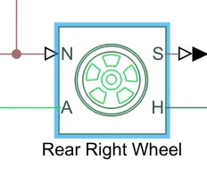
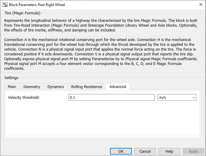
- Tire (magic formula) Block:-
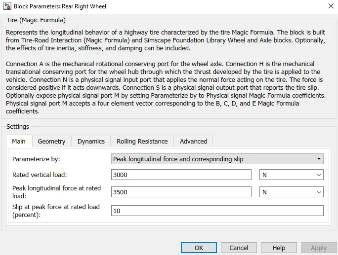
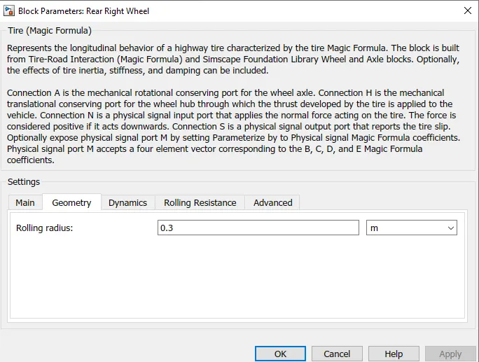
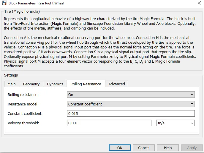
Represents the longitudinal behavior of a highway tire characterized by the tire Magic Formula. The block is built from Tire-Road Interaction (Magic Formula) and Simscape Foundation Library Wheel and Axle blocks. Optionally, the effects of tire inertia, stiffness, and damping can be included.
Connection A is the mechanical rotational conserving port for the wheel axle. Connection H is the mechanical translational conserving port for the wheel hub through which the thrust developed by the tire is applied to the vehicle. Connection N is a physical signal input port that applies the normal force acting on the tire. The force is considered positive if it acts downwards. Connection S is a physical signal output port that reports the tire slip. Optionally expose physical signal port M by setting Parameterize by to Physical signal Magic Formula coefficients. Physical signal port M accepts a four element vector corresponding to the B, C, D, and E Magic Formula coefficients.
- Parameters:-
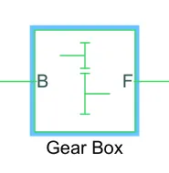
- GearBox Block:-
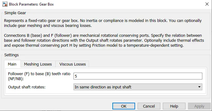
It is work as like Gearbox. Its Follower port is connected to the rear wheel axle to drive rear wheel and the base port is open to connect dc motor. In this we slected gear ratio is 5.
- Parameters:-
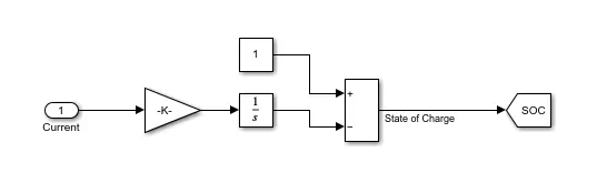
7] State of charge unit:-
8] Outcomes Unit:-
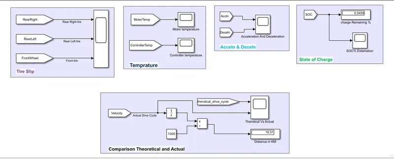
Results:-
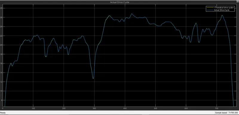
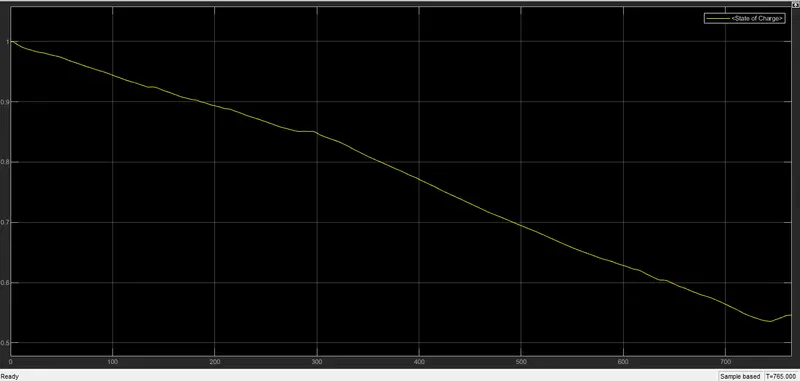
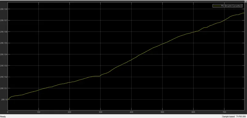
1] HWFET Drive Cycle (765 seconds):-
- Theoretical And actual Drive cycle:-
- State of charge:-
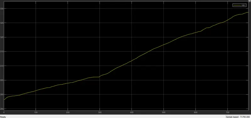
- Temperature of controller:-
- Temperature of motor:-
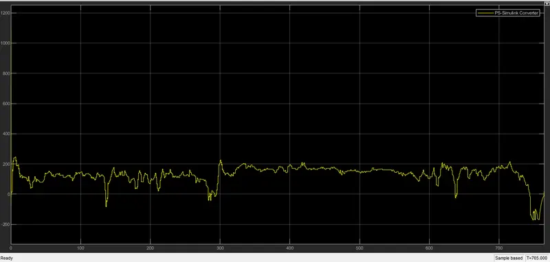
- Current Voltage:-
As we see in this graph the current voltage is suddenly increase at starting and it also decrease suddenly to 0 then it increase and going continuously in range of 0-200 A. As we see the maxm current voltage at normal driving condition is nearly 190-200 A. and during regenerative braking the current voltage is at -60 to -70A.
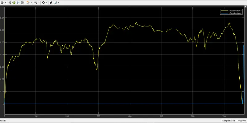
- Acceleration And Deceleration by driver:-
- Tire slip:-
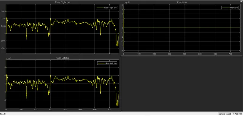
Result
2] Wide open throttle (100 km constant speed driving at 45 kmph):-
- Theoretical And actual Drive cycle:-
- State of charge:-
- Temperature of controller:-
- Temperature of motor:-
- Current Voltage:-
- Acceleration And Deceleration by driver:-
- Tire slip:-
It taking More time to running so cant upload result.
Result
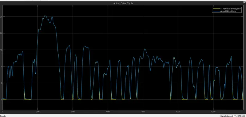
3] FTP 72 Drive Cycle (1372 seconds):- 13.13 km 0.718 remaining
- Theoretical And actual Drive cycle:-
As you see it is going equally to FTP 72 drive cycle and it is distance covered 13.13Km.
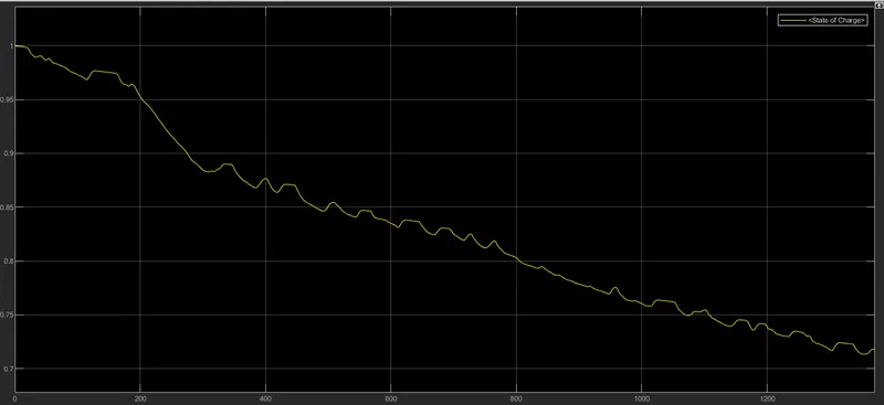
- State of charge:-
Using this cycle the charging was slowly decrease and in this regenerative braking many times occurs so the its continuosly charge. The nattery charging is only 29% and remaining 71%.
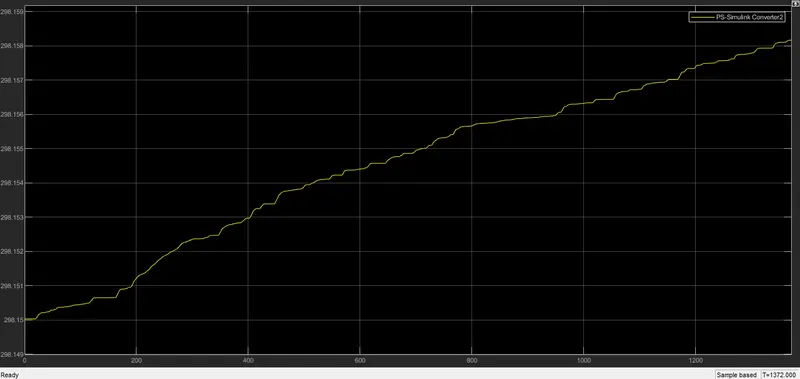
- Temperature of controller:-
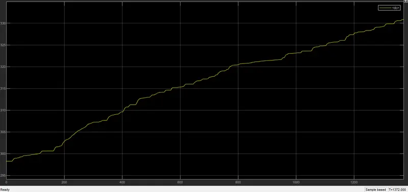
- Temperature of motor:-
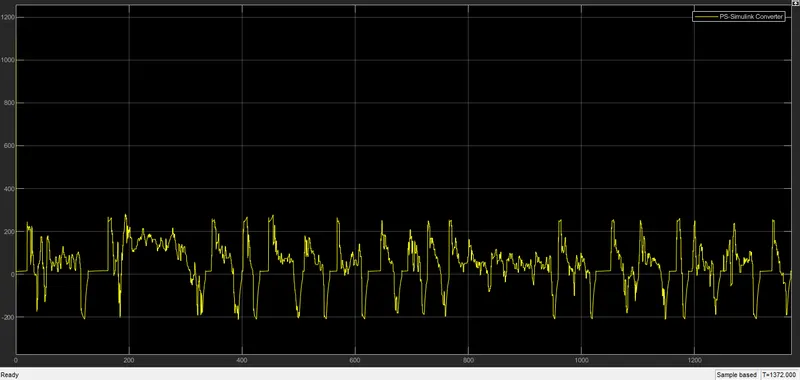
- Current Voltage:-
As you see the current flowing between in range -200 to 200. -200a is reegenerative braking applying.
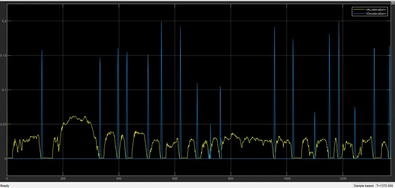
- Acceleration And Deceleration by driver:-
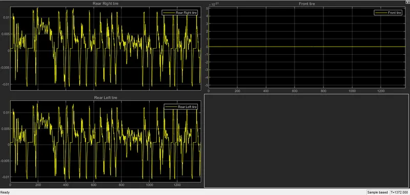
- Tire slip:-
Conclusion:-
| Drive Cycle | KM | SOC used | Motor Temp | Controller temp | Current |
| HWFET | 16.51 | 46% | 329 | 298.157 | 200 |
| FTP 72 | 13.13 | 29% | 331 | 298.158 | 250 |
Thank you
Dharmesh Bonde...