Final Project: Design of an Electric Vehicle

Design of an Electric Vehicle

AIM:

Create a MATLAB model of electric car which uses a battery and a DC motor. Choose suitable blocks from Powertrain block set. Prepare a report about your model including following:

Objectives:

1. System level configurations

2. Model parameters

3. Results

4. Conclusion

Introduction:

By 2030, the number of electric vehicles on the road is expected to increase from 3 million to 125 million, according to a prediction by the International Energy Agency. Due to the rising need for fossil fuels and pollution issues, that is almost 41 times greater than it is at the moment. Because of this, all major IC engine car manufacturers, including Ford and GM, are gradually shifting their focus to electric vehicles. In addition to the need from the market and customers for more affordable personal transportation, the government has begun to support electric vehicles through its regulations. Given all of these factors, it is essentially obvious that soon Electric Vehicles will be zooming all over our Highways.

The effects of this transformation have already started to emerge. Many successful electric vehicle manufacturers have developed in the last few years, including Tesla, Kia Soul, Navistar, and Kandi, to name a few. And as a result of these, there have also been numerous technological advances in the field of electric vehicle batteries and motors.

Electric Vehicle

A vehicle that can be propelled by an electric motor that draws power from a battery and can be charged externally is referred to as an EV. Instead of using gasoline, all-electric vehicles (also known as EVs or BEVs) contain a sizable battery that drives one or more electric motors. The current driving range of all-electric cars spans from 80 to more than 300 miles, with ranges getting further as new models are released. As comparison to gas-powered cars, all-electric vehicles require less maintenance in addition to avoiding the gas station.

All-electric vehicles are able to be charged at home using regular 120-volt or 240-volt house connections as well as away from the house at public or commercial charging stations. All-electric vehicles have one advantage over plug-in hybrids: the ability to employ DC fast charging, which can extend range by more than 100 miles in just 30 minutes.

The figure below shows the components of pure electric vehicle.

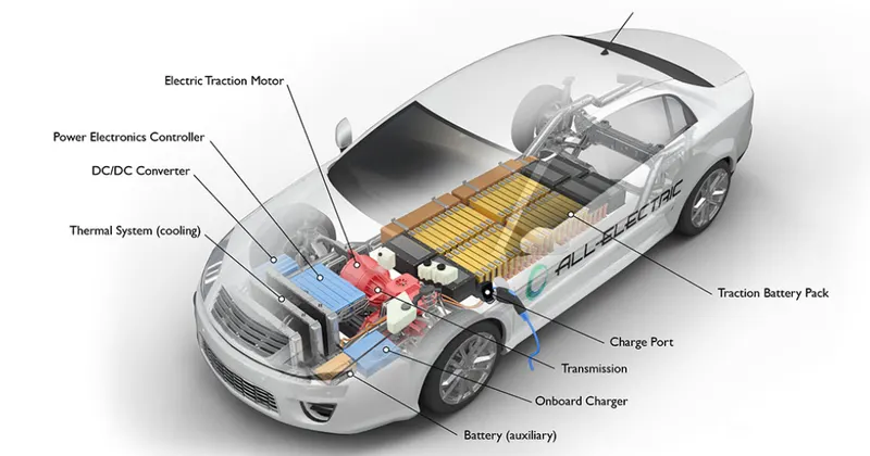
Key components of pure electric vehicle are

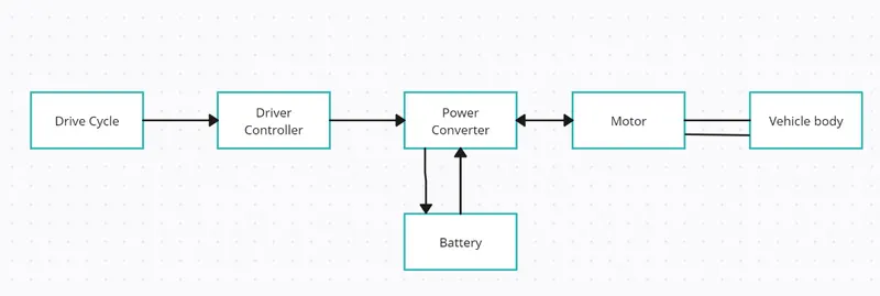
The figure below shows the block diagram of EV powertrain

MATLAB/SIMULINK model

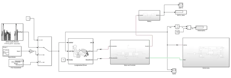
The EV powertrain is modeled using a Simulink model, as seen in the above figure. In this model, I've created an electric vehicle (EV) that operates using a variety of drive cycles, including FTP75, drive cycles created using signal builders, and drive cycles created using data from spreadsheets. These drive cycles are reference to the vehicle. This model includes a variety of subsystems, including "Battery," "Motor and Controller," and "Vehicle." Transmission, tire, and vehicle body are all parts of the vehicle's subsystems, where we can specify weight of vehicle, drag coefficient, frontal area, rolling resistance coefficient, and other characteristics. A DC motor and H-bridge controller are part of the Motor and Controller subsystem, which controls the motor in accordance with commands from the longitudinal driver block for acceleration or deceleration.Battery subsystem calculates a battery's state of charge (SOC) depending on usage, where discharged with the same amount of current input as the motor. The longitudinal driver block uses a PI controller that uses the vehicle's speed as feedback and attempts to match the reference speed by issuing the proper commands for braking or accelerating.

Sub-Systems

Vehicle Sub-systems

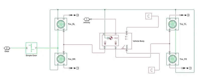
The above figure shows the vehicle subsystem where it contain different blocks like vehicle body block, 4 Tires blocks and Simple gear block. These blocks are connected in such a way that we can model a rear wheel drive vehicle.

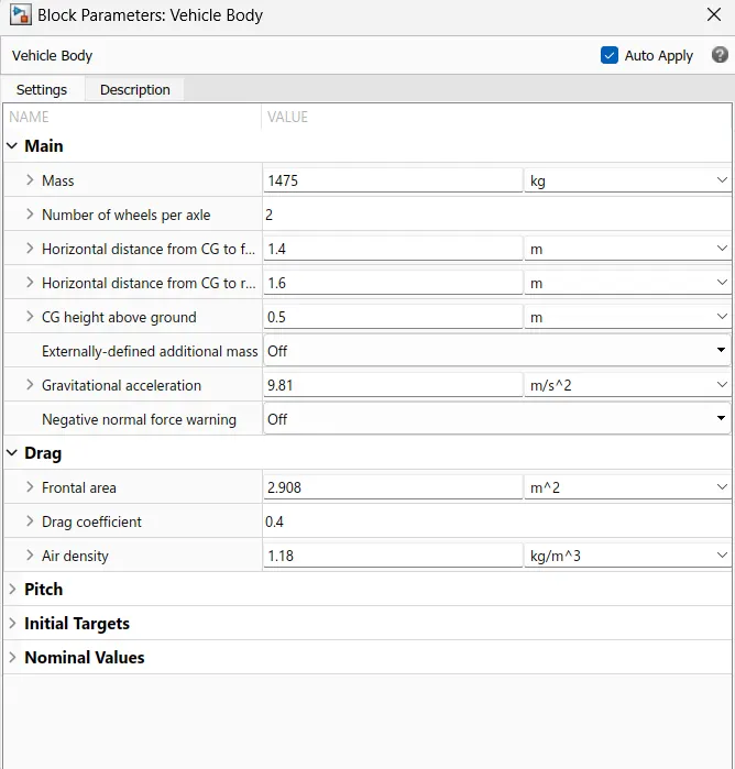
Vehicle body

It Represents a two-axle vehicle body in longitudinal motion. The block accounts for body mass, aerodynamic drag, road incline, and weight distribution between axles due to acceleration and road profile.

Connection H is the mechanical translational conserving port associated with the horizontal motion of the vehicle body. The resulting traction motion developed by tires should be connected to this port. Connections V, NF, and NR are physical signal output ports for vehicle velocity and front and rear normal wheel forces, respectively. Connections W and beta are physical signal input ports corresponding to headwind speed and road inclination angle, respectively.A constant zero input is given as head-wind & grade to the block.

Tire:

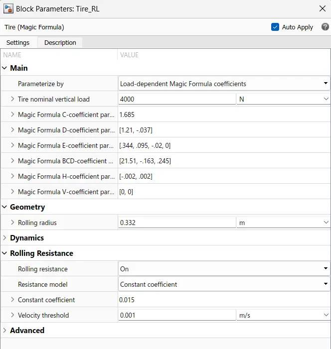
Represents the longitudinal behavior of a highway tire characterized by the tire Magic Formula. The block is built from Tire-Road Interaction (Magic Formula) and Simscape Foundation Library Wheel and Axle blocks. Optionally, the effects of tire inertia, stiffness, and damping can be included.

Connection A is the mechanical rotational conserving port for the wheel axle. Connection H is the mechanical translational conserving port for the wheel hub through which the thrust developed by the tire is applied to the vehicle. Connection N is a physical signal input port that applies the normal force acting on the tire. Connection S is a physical signal output port that reports the tire slip.

Simple Gear:

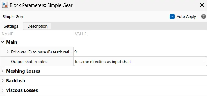
Represents a fixed-ratio gear or gear box. No inertia or compliance is modeled in this block. We can optionally include gear meshing, backlash, and viscous bearing losses.

Connections B (base) and F (follower) are mechanical rotational conserving ports. Specify the relation between base and follower rotation directions with the Output shaft rotates parameter. Optionally include thermal effects and expose thermal conserving port H by setting Friction model to a temperature-dependent setting.

Chosen Parameters

Weight - 1475 kg

Front area - 2.908

Rolling radius - 0.332, it is calculated from referring the tyre size of tata nexon ev

Rolling resistant coefficient - 0.015

Rest of the parameters are kept as default

Motor and Controller Sub-System

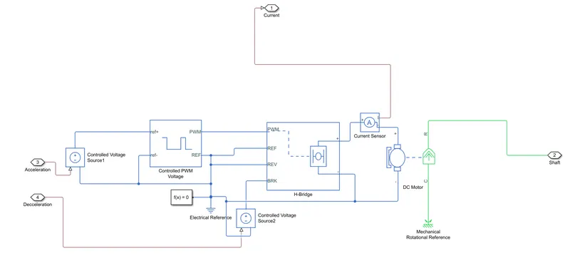
The above figure shows the vehicle subsystem where it contain different blocks like DC Motor, H-Bridge, Controlled PWM Voltage, current sensor, Controlled Voltage sources and references etc.

The input to this Sub system is acceleration and deceleration commant from the driver. The output is mechanical rotational port, which is associated with rotor of DC motor. The current output gives the current through the DC motor. This motor with act as a generator during the time of regenerative braking.

DC motor:

This block represents the electrical and torque characteristics of a DC motor.When a positive current flows from the electrical + to - ports, a positive torque acts from the mechanical C to R ports.

Here Under Electrical Torque, We choose Field type as Permanent Magnet, Model Parameterrization is by rated load and speed.

Assumtion

Rated torque is 245 , motor efficiency is 95% and rated load(mechanical power) is 94 Kw. Using we calculated the rated speed as 3860 rpm

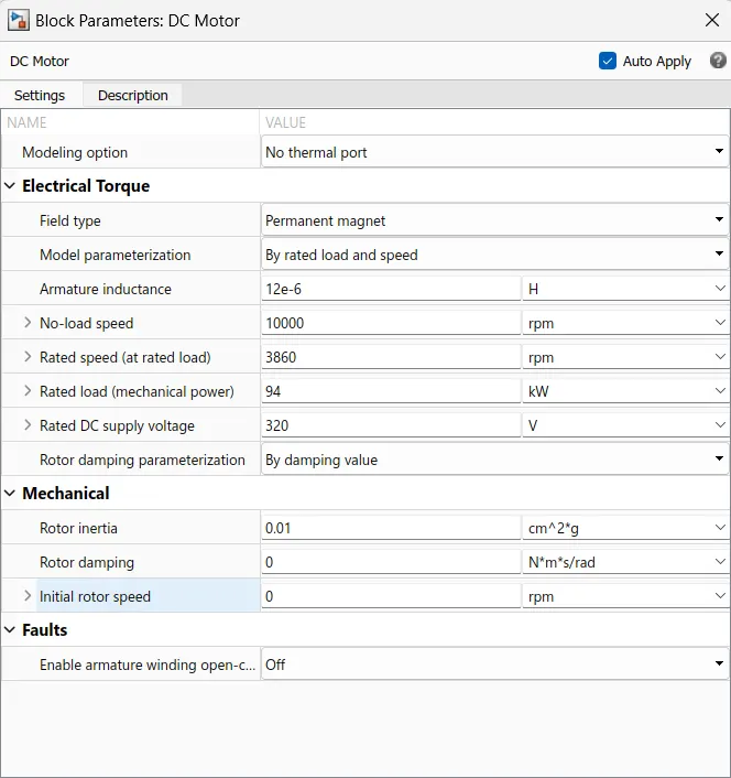
Chosen Parameter

No load speed = 10000 rpm

Rated speed = 3860 rpm

Rated load(Mechanical power) = 94 kW

Rated DC supply voltage = 320 V

Rest of the parameter is kept as default.

H-Bridge

This block represents an H-bridge motor drive. This block control the power to motor based on the load requirement.

The block can be driven by the Controlled PWM Voltage block in PWM or Averaged mode. In PWM mode, the motor is powered if the PWM port voltage is above the Enable threshold voltage. In Averaged mode, the PWM port voltage divided by the PWM signal amplitude parameter defines the ratio of the on-time to the PWM period. Using this ratio and assumptions about the load, the block applies an average voltage to the load that achieves the correct average load current. The Simulation mode parameter value must be the same for the Controlled PWM Voltage and H-Bridge blocks.

In H-bridge block we kept power supply is internal. Simulation mode is configured as ‘Averaged’ to achieve fast simulation. Regenerative braking is also enabled.

A controlled voltage is connected to Brake(BRK) port, it produce a voltage according to the deceleration command from the driver

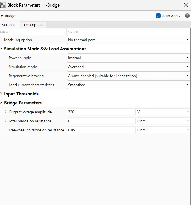
chosenParameter

Output voltage amplitude = 320 V , same as rated motor voltage

All other parameters are set as default

Controlled PWM Voltage

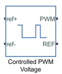
This block creates a Pulse-Width Modulated (PWM) voltage across the PWM and REF ports. The output voltage is zero when the pulse is low, and is equal to the Output voltage amplitude parameter when high. Duty cycle is set by the input value. The PWM signal created according to input acceleration commant, is given as a input to the H-Bridge block.

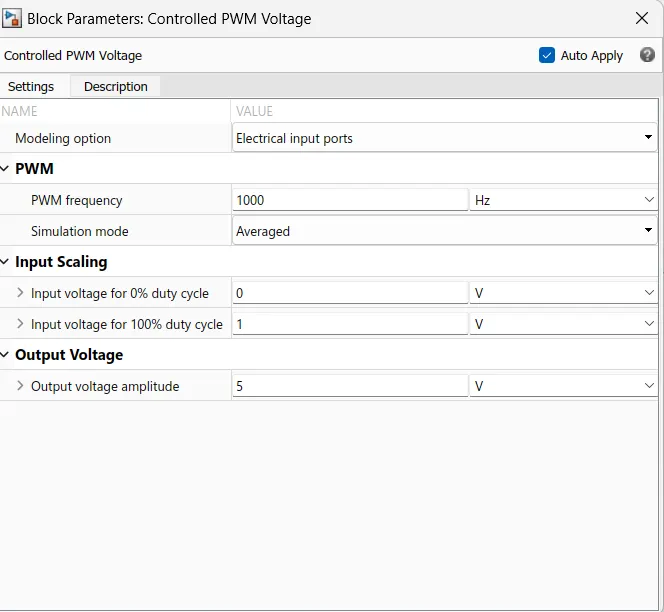
The Simulation mode can be set to PWM or Averaged. In PWM mode, the output is a PWM signal. In Averaged mode, the output is constant with value equal to the averaged PWM signal.

Here all the parameters is kept as default.

Controlled Voltage Source

The Controlled Voltage Source block represents an ideal voltage source that is powerful enough to maintain the specified voltage at its output regardless of the current flowing through the source.

The block has one physical signal input port and two electrical conserving ports associated with its electrical terminals.

Battery Subsystem

This subsystem models the battery for EV such it takes motor current as input and outputs the SOC of battery. During regenerative braking this battery charges. The figure below shows the battery subsystems

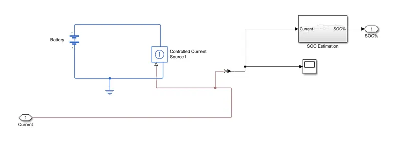
Battery

This block models a battery. If you select Infinite for the Battery charge capacity parameter, the block models the battery as a series internal resistance and a constant voltage source. If you select Finite for the Battery charge capacity parameter, the block models the battery as a series internal resistance plus a charge-dependent voltage source defined by:

V = Vnom*SOC/(1-beta*(1-SOC))

where SOC is the state of charge and Vnom is the nominal voltage. Coefficient beta is calculated to satisfy a user-defined data point [AH1,V1].

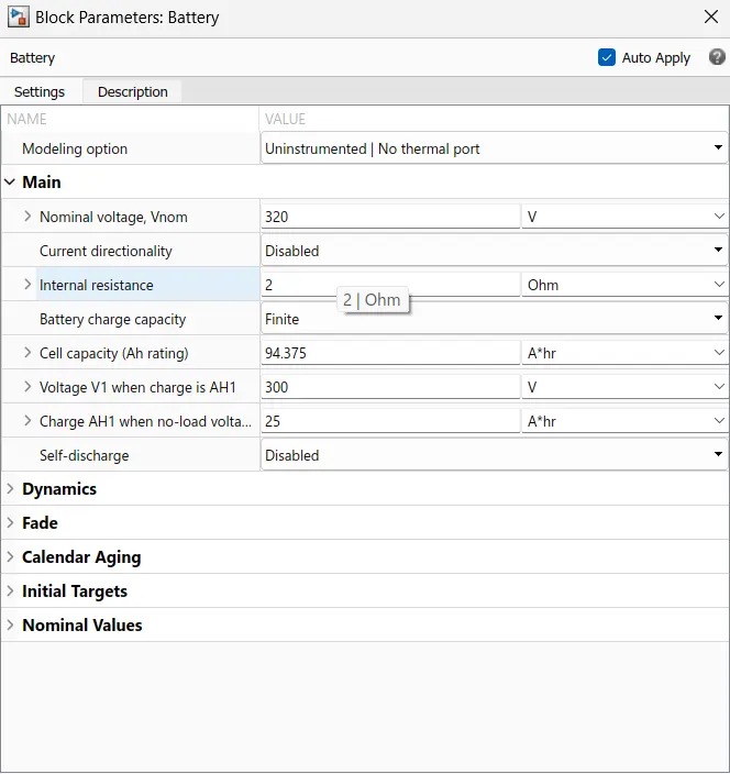
Here we assume 30kWh battery pack

Parameters

Battery charge capacity is fine

Nominal Voltage = 320V

Battery capacity = 94.375 Ah

Rest of the parameters is set as default

SOC Estimation

For estimation of the SOC (State of Charge) of battery we have to create a subsystem where it estimate the SOC of battery using coulomb counting method. This subsystem consist of Rate transition, Gain, Discrete Time Integrator, Constant and Sum blocks.

We assume initial SOC is 100%. and battery capacity 94.375 Ah.

The figure below shows the subsystem

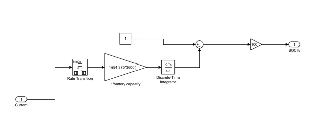
The input to this subsystem is current and outputs the SOC.

The Rate Transition block transfers data from the output of a block operating at one rate to the input of a block operating at a different rate.

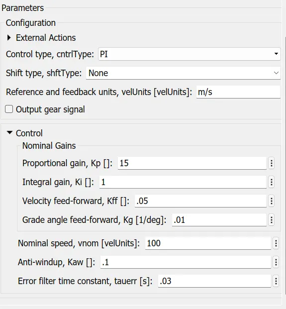
Longitudinal Driver

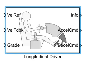
It is aparametric longitudinal speed tracking controller for generating normalized acceleration and braking commands based on reference and feedback velocities.

The input to this block is Reference velocity, feedback velocity and Grade and it outputs the acceleration and deceleration commands.

The Reference input velocity is obtained from drive cycle data. it contain a controller where it outputs neccesary acceleration and deceleration based on the its inputs.

Multiport Switch

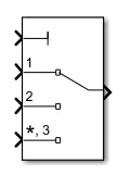
This block accept different inputs and outputs only one at a time. With help of this switch we can give different input to the longitudinal driver so that we can observe the performance for each case

Drive Cycle inputs

In this model we use three different drive cycle inputs. They are:

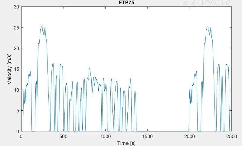
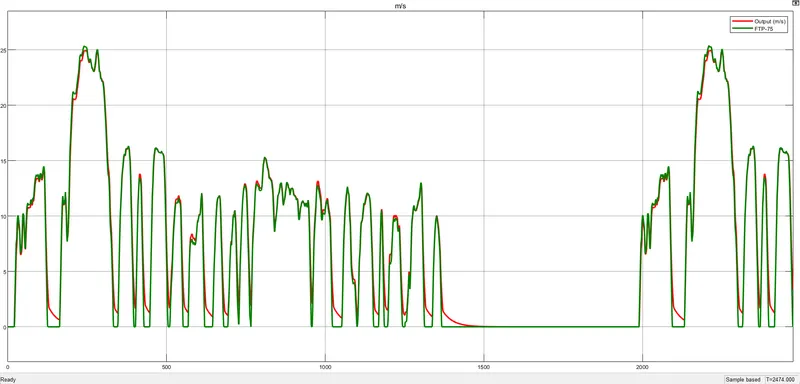
FTP-75 Drive cycle

Simulation is done for 2474 sec

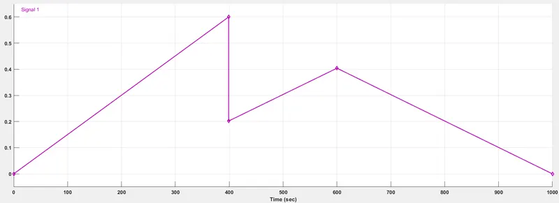
Drive cycle built by signal builder

Simulation is done for 1000 sec

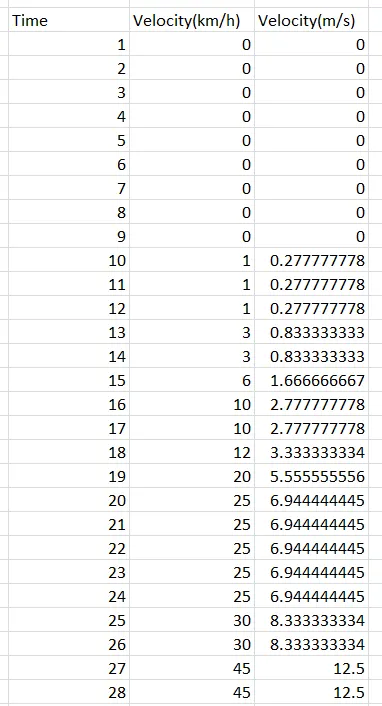
Drive cycle built from spread sheet data

The simulation done for 120 sec, The entire spread sheet is attached along with this.

Simulation and Results

Here the simulating is done using the selected the drive cycle and result is analysed

Case-1: FTP-75 Drive cycle

Here simualtion time is set as 2474 sec

Result

Speed

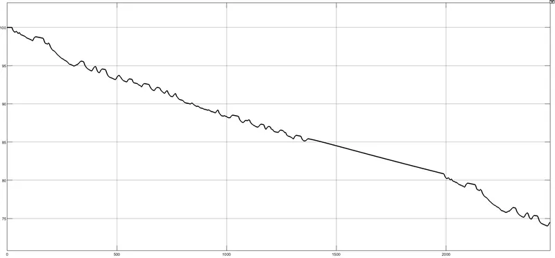
SOC %

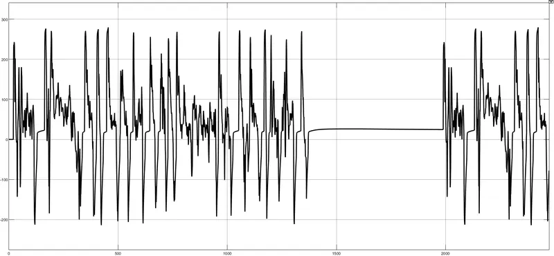
Current from Battery

Observation

battery SOC at end of the cycle = 74.51%

Distance coverd = 18.62 km

From the above result we can observe that Vehicle almost follow the reference input and vehicle achieved a top speed of 25 m/s(90 kmph). But during the deceleration we can see vehicle not exactly following the reference, it is

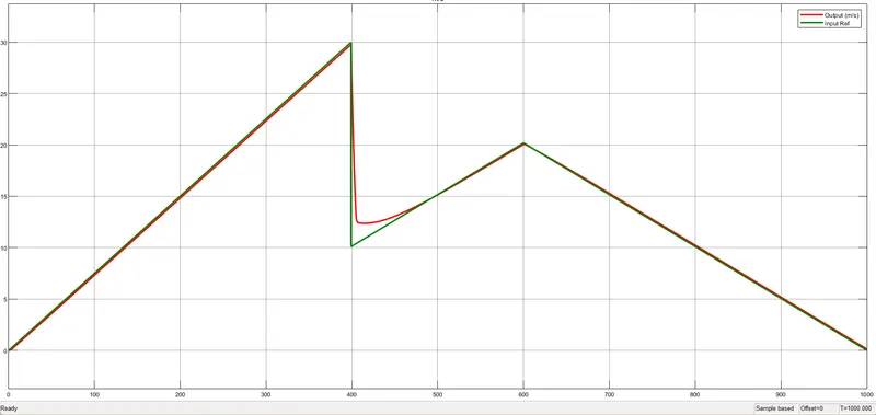
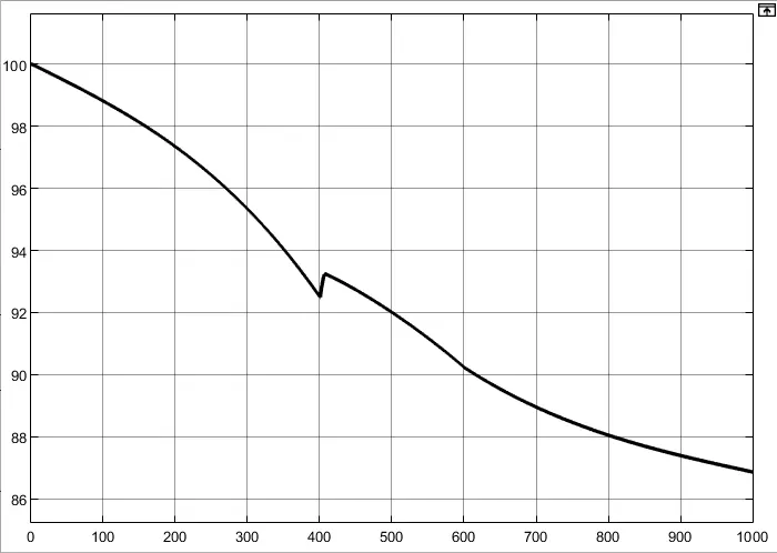
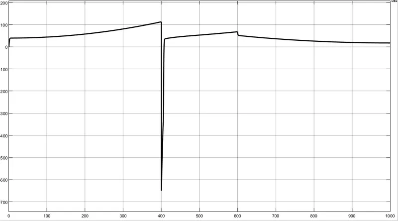
Case-2: Drive cycle built by signal builder

Result

Speed

SOC %

Current

Observation

Battery SOC at end of the cycle = 86.86%

Distance coverd = 13.05 km

From the above result we can see Vehicle almost follow the input reference and during deceleration time, the battery not charging properly. it is because of very low deceleration rate.

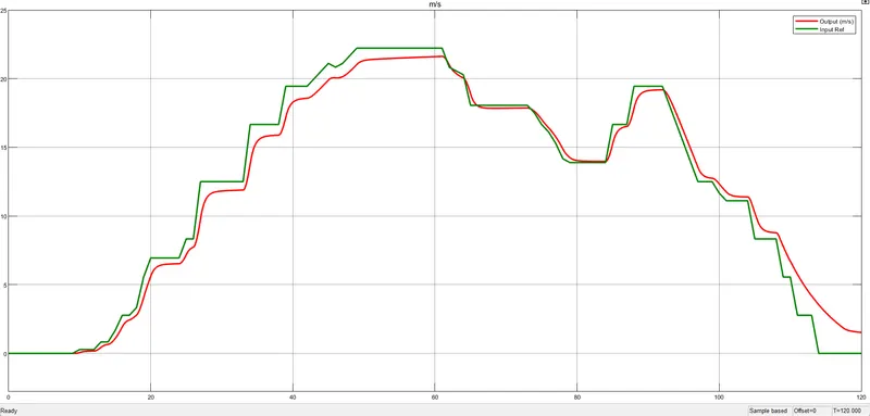
Case-3: Drive cycle built from spread sheet data

Result

Speed

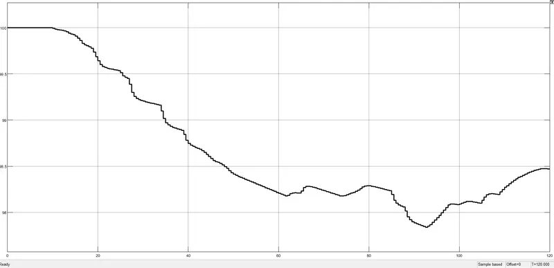
SOC %

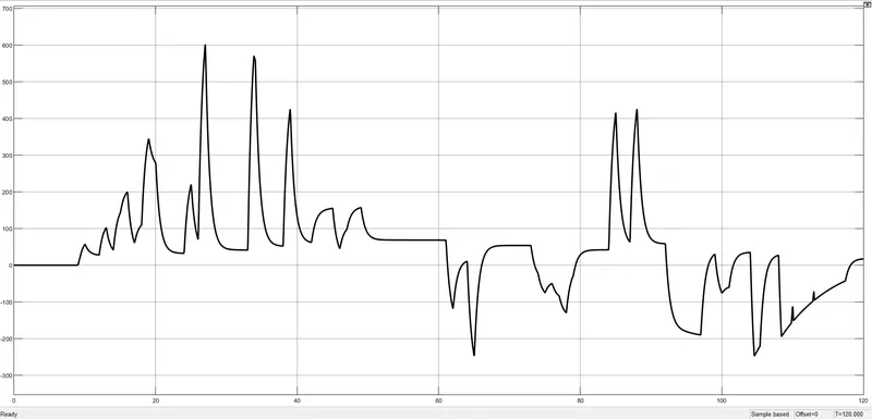
Current from Battery

Observation

Battery SOC at end of the cycle = 98.47%

Distance coverd = 1.465 km

From the above result we can say that the vehicle is almost following the reference input and battery is charging during the time deceleration.

Conclusion-

• Created a MATLAB model of electric car which uses a battery and a DC motor and analysed the performance of vehicle with different inputs.
• It observed that vehicle almost following the reference input, Battery SOC decreases during the acceleration time and battery charges during deceleration time.
• The modelled EV is rear wheel drive, Battery SOC is calculated based on coulomb counting method and reference inputs used are FTP-75 Drive cycle, Signal builder, and drive cycle using a spread sheet.

References

• https://skill-lync.com/knowledgebase/modeling-of-vehicle-body-and-tires
• https://nexonev.tatamotors.com/features/
• Modeling of Electric Vehicles using MATLAB & Simulink - (Part-1) - YouTube

File link -

Model- https://drive.google.com/file/d/1sKB2K5wvBRXKP3X8D3v4BtcFcXlsYteA/view?usp=share_link

Spread sheet Drive cycle- https://docs.google.com/spreadsheets/d/17yDYE8XvovJ-Hq4KGdsQf4-IQNJLZbLa/edit?usp=share_link&ouid=105049652077660954312&rtpof=true&sd=true