Final Project: Design of an Electric Vehicle

Design of an Electric Vehicle:

Objectives:

Create a MATLAB model of electric car which uses a battery and a DC motor. Choose suitable blocks from Powertrain block set. Prepare a report about your model including following:

• System level configurations
• Model parameters
• Results
• Conclusion

Introduction:

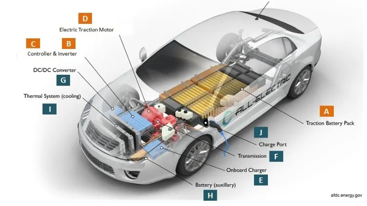
An electric vehicle (EV) is one that operates on an electric motor, instead of an internal-combustion engine that generates power by burning a mix of fuel and gases. Therefore, such as vehicle is seen as a possible replacement for current-generation automobile, in order to address the issue of rising pollution, global warming, depleting natural resources, etc. Though the concept of electric vehicles has been around for a long time, it has drawn a considerable amount of interest in the past decade amid a rising carbon footprint and other environmental impacts of fuel-based vehicles.

Battery

The battery of an electric car can be charged through the use of ordinary grid electricity at a specialized power station. But aside from the conventional lithium-ion battery technologies, there are also other major battery technologies which can be used for electric cars.

Lithium-Ion Batteries: This battery technology gives extra performance and range. However, it also carries the highest price tag. Lithium-ion batteries are lighter than Lead acid and Nickel metal. These are also the batteries used in digital cameras and smartphones.

Lead Acid Batteries: This battery technology is the most popular. It is also the cheapest among the battery technologies. What’s good about it is it’s 97% recyclable.

Nickel Metal Hydride Batteries: This battery technology provides higher output and better performance but it costs much more than lead-acid batteries.

Motor Controller

The motor controller of an electric car administers its complete operation and the distribution of its power at any given moment. It acts as a floodgate between the motor and batteries. It helps monitor and regulates all key performance indications such as the vehicle’s operator, motor, battery, and accelerator pedal. It has a microprocessor which can limit or redirect current. It is used to either improve the mechanical performance of the car or suit the operator’s driving style. There are also more refined controllers which are capable of greater accuracy and thus, higher efficiency.

Regenerative Braking

As the electric car moves, the electric motor generates a forward momentum and it can be used to charge the batteries when you apply the brakes, which is commonly referred to as regenerative braking. It can recover up to about fifteen percent of used energy for acceleration. Though this component is indeed effective, it cannot generate enough to fully recharge an electric car.

Drive System

• The function of the drive system is to transfer mechanical energy to the traction wheels, generating motion. An electric car does not require a conventional transmission. However, it has several internal configurations depending on the components in use. For example, there are some designs which use multiple smaller motors that power each wheel individually. Large electric motors, on the other hand, may be coupled to the rear wheels using a differential housing.
• The components of an electric powered car are much simpler compared to the components of a gasoline-powered car engine. However, electric cars cannot go as fast as gasoline-powered cars can. Electric vehicles, on the other hand, can reduce energy consumption in different ways like automatically turning the engine off when the car is idle.

Simulink Model:

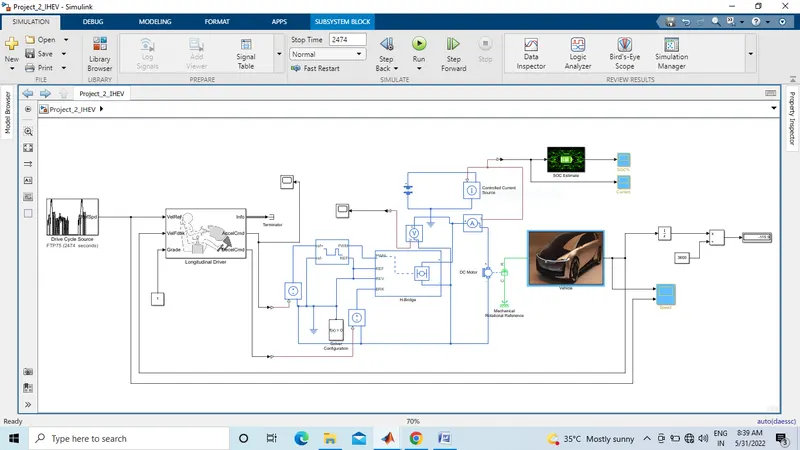
Model Description:

Drive Cycle Source:

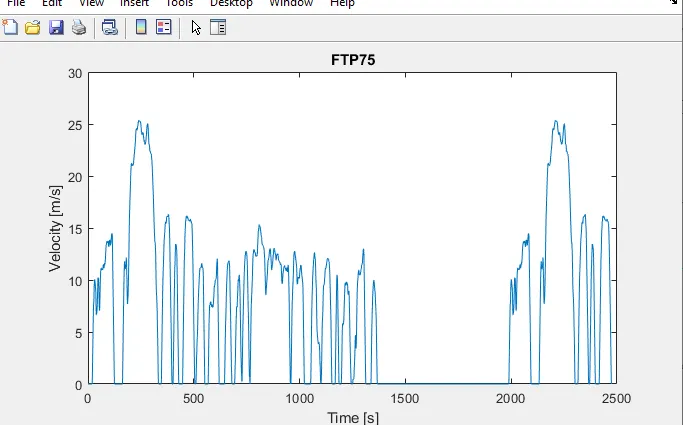
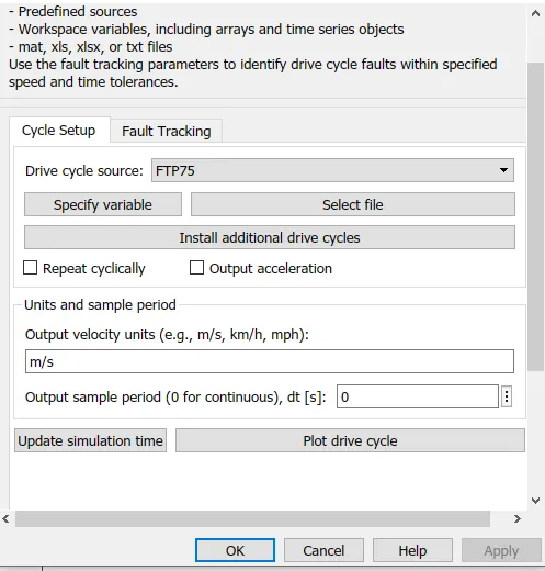
The Drive Cycle Source block generates a standard or user-specified longitudinal drive cycle. The block output is the specified vehicle longitudinal speed, which you can use to:

• Predict the engine torque and fuel consumption that a vehicle requires to achieve desired speed and acceleration for a given gear shift reference.
• Produce realistic velocity and shift references for closed loop acceleration and braking commands for vehicle control and plant models.
• Study, tune, and optimize vehicle control, system performance, and system robustness over multiple drive cycles.
• Identify the faults within tolerances specified by standardized tests, including:
• EPA dynamometer driving schedules¹
• Worldwide Harmonised Light Vehicle Test Procedure (WLTP) laboratory tests .

Vehicle:

This is a subsystem of vehicle included vehicle body , tire and gear box.

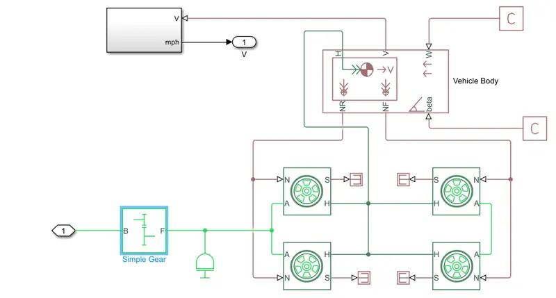
Vehicle Body:

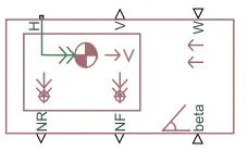
• The Vehicle Bodyblock represents a two-axle vehicle body in longitudinal motion. The vehicle can have the same or a different number of wheels on each axle. For example, two wheels on the front axle and one wheel on the rear axle. The vehicle wheels are assumed identical in size. The vehicle can also have a center of gravity (CG) that is at or below the plane of travel.
• The block accounts for body mass, aerodynamic drag, road incline, and weight distribution between axles due to acceleration and road profile. Optionally include pitch and suspension dynamics. The vehicle does not move vertically relative to the ground.
• The block has an option to include an externally-defined mass and an externally-defined inertia. The mass, inertia, and center of gravity of the vehicle body can vary over the course of simulation in response to system changes.

W — Headwind speed, m/s

beta — Road incline angle, rad

CG — Center of gravity, m two-element vector

M — Mass, kg

J — External moment of inertia, kg*m^2

V — Longitudinal velocity, m/s
NF — Front axle normal force, N

NR — Rear axle normal force, N
H — Horizontal motion mechanical translational

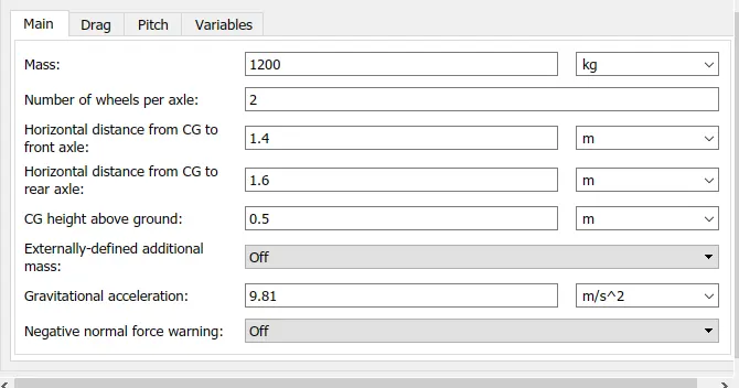
Fig: Vehicle body Parameters

Tire:

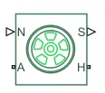
• The Tire (Magic Formula)block models a tire with longitudinal behavior given by the Magic Formula [1], an empirical equation based on four fitting coefficients. The block can model tire dynamics under constant or variable pavement conditions.
• The longitudinal direction of the tire is the same as its direction of motion as it rolls on pavement. This block is a structural component based on the Tire-Road Interaction (Magic Formula)
• To increase the fidelity of the tire model, you can specify properties such as tire compliance, inertia, and rolling resistance. However, these properties increase the complexity of the tire model and can slow down simulation. Consider ignoring tire compliance and inertia if simulating the model in real time or if preparing the model for hardware-in-the-loop (HIL) simulation.

N — Normal force
M — Magic formula coefficients
S — Slip
A — Axle mechanical rotational

H — Hub mechanical translational

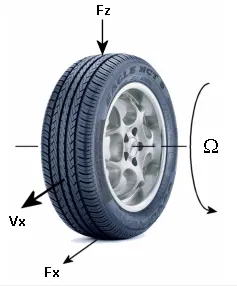
The Tire (Magic Formula) block models the tire as a rigid wheel-tire combination in contact with the road and subject to slip. When torque is applied to the wheel axle, the tire pushes on the ground (while subject to contact friction) and transfers the resulting reaction as a force back on the wheel. This action pushes the wheel forward or backward. If you include the optional tire compliance, the tire also flexibly deforms under load.

The figure shows the forces acting on the tire. The table defines the tire model variables.

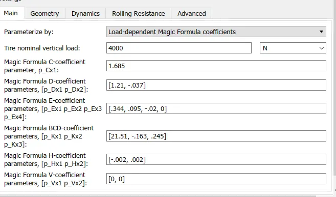
Fig: Tire Parameters.

Simple Gear:

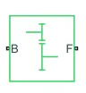
The Simple Gear block represents a gearbox that constrains the connected driveline axes of the base gear, B, and the follower gear, F, to corotate with a fixed ratio that you specify. You choose whether the follower axis rotates in the same or opposite direction as the base axis. If they rotate in the same direction, the angular velocity of the follower, ωF, and the angular velocity of the base, ωB, have the same sign. If they rotate in opposite directions, ωF and ωB have opposite signs. You can easily add and remove backlash, faults, and thermal effects.

T — External fault trigger
B — Base rotational mechanical

F — Follower rotational mechanical

H — Heat flow

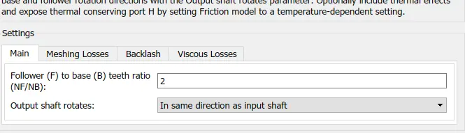
Fig: Simple Gear Parameters

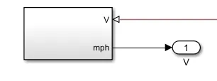
For Velocity calculation I made this model. I used ps simulink converter , gain block , zero order hold and outport block.

Inertia:

Ideal mechanical rotational inertia

The Inertia block represents an ideal mechanical translational inertia that is described with the following equation:

T=Jdω/dt

where:

T is inertia torque.

J is inertia.

ω is angular velocity.

t is time.

• By default, the block has one mechanical translational conserving port. The block positive direction is from its port to the reference point. This means that the inertia torque is positive if inertia is accelerated in the positive direction.
• In some applications, it is customary to display inertia in series with other elements in the block diagram layout. To support this use case, the Number of graphical portsparameter lets you display a second port on the opposite side of the block icon. The two-port variant is purely graphical: the two ports have the same angular velocity, so the block functions exactly the same whether it has one or two ports. The block icon changes depending on the value of the Number of graphical ports

I — Port that connects inertia to the circuit
J — Second graphical port

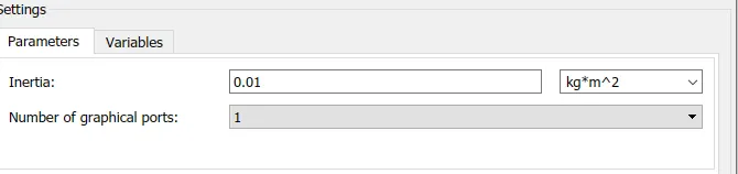
Fig: Inertia Parameters.

PS Terminator:

Use this block to terminate physical signal outputs. Unconnected physical signal output ports do not generate warnings, but connection to a PS Terminator can be used to indicate that the signal was not inadvertently left unconnected

PS Constant: This block creates a physical signal constant

Longitudinal Driver:

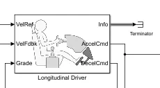
The Longitudinal Driver block implements a longitudinal speed-tracking controller. Based on reference and feedback velocities, the block generates normalized acceleration and braking commands that can vary from 0 through 1. You can use the block to model the dynamic response of a driver or to generate the commands necessary to track a longitudinal drive cycle.

VelRef — Reference vehicle velocity

EnblAccelOvr — Enable acceleration command override

AccelOvrCmd — Acceleration override command

AccelHld — Acceleration hold
scalar

AccelZero — Disable acceleration command

EnblDecelOvr — Enable deceleration command override

DecelOvrCmd — Deceleration override command

DecelHld — Deceleration hold

DecelZero — Disable deceleration command

ExtGear — Gear

VelFdbk — Longitudinal vehicle velocity

Grade — Road grade angle

Info — Bus signal

AccelCmd — Commanded vehicle acceleration

DecelCmd — Commanded vehicle deceleration

GearCmd — Commanded vehicle gear

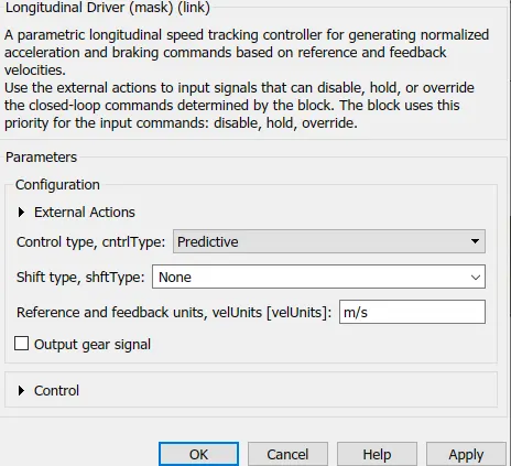
Fig: Longitudinal Driver Parameters.

Controlled PWM Voltage:

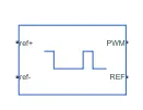
The Controlled PWM Voltage block represents a pulse-width modulated (PWM) voltage source. The block has two modeling variants, accessible by right-clicking the block in your block diagram and then selecting the appropriate option from the context menu, under Simscape > Block choices:

The model is based on the following assumptions:

• The REF output of this block is floating, it is not tied to the Electrical Reference. One consequence of this is that if you connect the PWM and REF electrical ports directly to the PWM and REF electrical ports of an H-bridge or a gate driver, you must attach an Electrical Referenceblock to the REF connection line.
• Do not connect the Controlled PWMblock directly to a semiconductor gate, because this omits the gate driver output impedance that determines switching dynamics. Use a Gate Driver or a Half-Bridge Driver block to set the gate-source or the gate-emitter voltage.
• Do not use the Controlled PWMblock to drive a motor block directly. A PWM motor driver goes open circuit in between pulses. Use the H-Bridge block to drive a motor block.
• When driving a motor via the H-Bridgeblock, set the Simulation mode parameter to Averaged to speed up simulations. You must also set the Simulation mode parameter of the H-Bridge block to Averaged This applies the average of the demanded PWM voltage to the motor. The Averaged mode assumes that the impedance of the motor inductive term is small at the PWM frequency. To verify this assumption, run the simulation using the PWM mode and compare the results to those obtained from using the Averaged mode.
• If you are linearizing your model, set the Simulation modeparameter to Averaged and ensure that you have specified the operating point of the block correctly. You can only linearize the block for inputs corresponding to a duty cycle greater than zero and less than 100 percent.
• When you use this block in PWMmode with the Use local solver option selected in the Solver Configuration block, set the Switching event type parameter to Discrete—time – Best for fixed-step solvers. Using the Asynchronous – Best for variable-step solvers option in this situation may produce inaccuracies, because simulation with the local solver implies fixed step, and the PWM events will not always coincide precisely with the simulation steps. This results in PWM events sometimes occurring one simulation step late.

u — Control signal, unitless
ref+ — Positive terminal
ref- — Negative terminal
PWM — Pulse-width modulated signal
REF — Floating zero volt reference

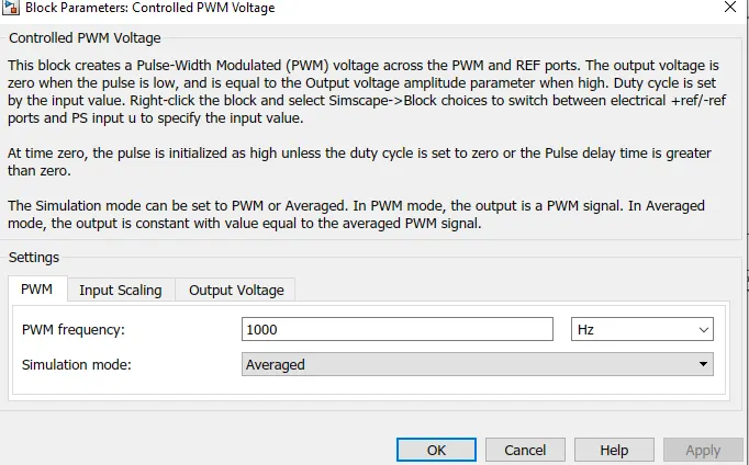
Fig: Controlled PWM Voltage.

H-bridge:

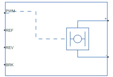
The H-Bridge block represents an H-bridge motor driver. The block has the following two Simulation mode options:

PWM — The H-Bridge block output is a controlled voltage that depends on the input signal at the PWM port. If the input signal has a value greater than the Enable threshold voltage parameter value, the H-Bridge block output is on and has a value equal to the value of the Output voltage amplitude parameter. If it has a value less than the Enable threshold voltage parameter value, the block maintains the load circuit using one of the following three Freewheeling mode options:

• Via one semiconductor switch and one freewheeling diode
• Via two freewheeling diodes
• Via two semiconductor switches and one freewheeling diode
• The first and third options are sometimes referred to as synchronous operation.

The signal at the REV port determines the polarity of the output. If the value of the signal at the REV port is less than the value of the Reverse threshold voltage parameter, the output has positive polarity; otherwise, it has negative polarity.

Averaged — This mode has two Load current characteristics options:

Smoothed

Unsmoothed or discontinuous.

V+ — Positive supply connection

V- — Negative supply connection

PWM — Pulse-width modulated signal

REF — Reference

REV — REV

BRK — BRK

H — Thermal port

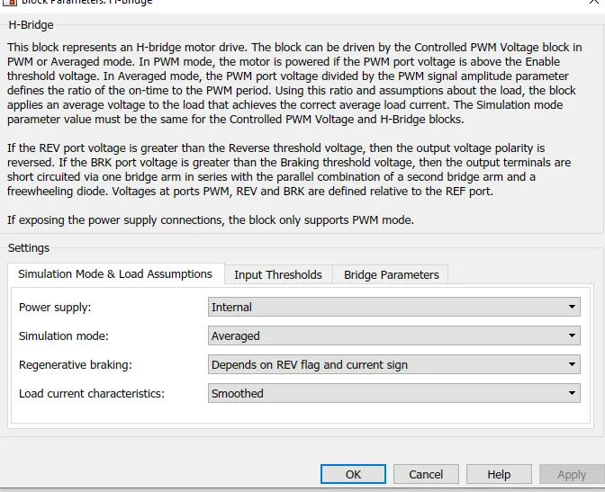
Fig: Parameters of H.bridge

DC Motor:

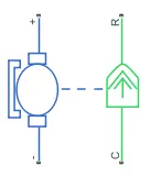
The DC Motor block represents the electrical and torque characteristics of a DC motor using the following equivalent circuit model:

You specify the equivalent circuit parameters for this model when you set the Model parameterization parameter to By equivalent circuit parameters. The resistor R corresponds to the resistance you specify in the Armature resistance parameter. The inductor L corresponds to the inductance you specify in the Armature inductance parameter.

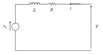
You can specify how to generate the magnetic field of the DC motor by setting the Field type parameter to the desired option. The permanent magnets in the motor induce the following back emf v_b in the armature:

+ — Positive terminal

- — Negative terminal

C — Motor case

R — Motor rotor

F+ — Positive field

F- — Negative field

Fig: DC motors Parameters.

SOC Estimate:

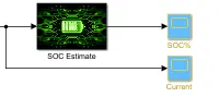
This is a subsystem block . this subsystem block calculate the how much battery charge available after vehicle travel any certain distance.

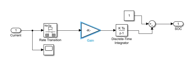
I used one input port. Then connect a rate transition block. Then connect gain block and connect a discrete time integrator block . then connect a sum block .then connect a soc block

Gain block value-

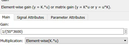
And all other parameters are default state.

Usages Others Block:

Control Voltage source:- The block represents an ideal voltage source that is powerful enough to maintain the specified voltage at its output regardless of the current passing through it. The output voltage is V = Vs, where Vs is the numerical value presented at the physical signal port.

Voltage Sensor:- The block represents an ideal voltage sensor, that is, a device that converts voltage measured between any electrical connections into a physical signal proportional to the voltage.

Connections + and - are conserving electrical ports through which the sensor is connected to the circuit. Connection V is a physical signal port that outputs voltage value.

Control Current Souce:- The block represents an ideal current source that is powerful enough to maintain the specified current through it regardless of the voltage across it. The output current is I = Is, where Is is the numerical value presented at the physical signal port.

Current Sensor:- The block represents an ideal current sensor, that is, a device that converts current measured in any electrical branch into a physical signal proportional to the current.

Connections + and - are conserving electrical ports through which the sensor is inserted into the circuit. Connection I is a physical signal port that outputs current value.

Electric Reference:- Electrical reference port. A model must contain at least one electrical reference port (electrical ground).

Solver Configuration:- Defines solver settings to use for simulation.

Battery:

The Battery block represents a simple battery model. The block has four modeling variants, accessible by right-clicking the block in your block diagram and then selecting the appropriate option from the context menu, under Simscape > Block choices:

• Uninstrumented | No thermal port— Basic model that does not output battery charge level or simulate thermal effects. This modeling variant is the default.
• Uninstrumented | Show thermal port— Model with exposed thermal port. This model does not measure internal charge level of the battery.
• Instrumented | No thermal port— Model with exposed charge output port. This model does not simulate thermal effects.

Instrumented | Show thermal port — Model that lets you measure internal charge level of the battery and simulate thermal effects. Both the thermal port and the charge output port are exposed.

The instrumented variants have an extra physical signal port that outputs the internal state of charge. Use this functionality to change load behavior as a function of state of charge, without the complexity of building a charge state estimator.

The thermal port variants expose a thermal port, which represents the battery thermal mass. When you select this option, provide additional parameters to define battery behavior at a second temperature. For more information, see Modeling Thermal Effects.

The battery equivalent circuit is made up of the fundamental battery model, the self-discharge resistance RSD, the charge dynamics model, and the series resistance R0.

Rate Transition:- The Rate Transition block transfers data from the output of a block operating at one rate to the input of a block operating at a different rate. Use the block parameters to trade data integrity and deterministic transfer for faster response or lower memory requirements. To learn about data integrity and deterministic data transfer, see Data Transfer Problems (Simulink Coder).

Discrete-Time Integrator:-

Use the Discrete-Time Integrator block in place of the Integrator block to create a purely discrete model. With the Discrete-Time Integrator block, you can:

• Define initial conditions on the block dialog box or as input to the block
• Define an input gain (K) value
• Output the block state
• Define upper and lower limits on the integral
• Reset the state with an additional reset input

Output Result:

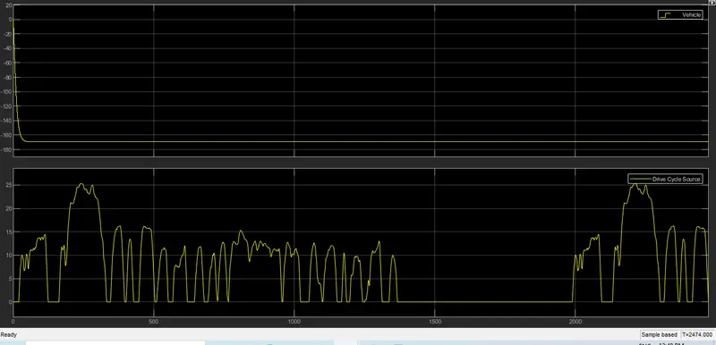
According FTP drive cycle and simulation time is 2474 sec. after 2474 sec vehicle travel aprx 116 km. drive cycle graph shown above with vehicle speed graph.

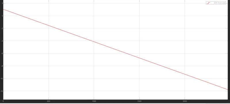
SOC% graph after travel the vehicle.

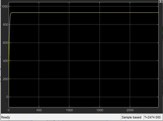
Supply current by the battery pack.

Conclusion:

I used FTP drive cycle for check the vehicle driving cycle condition. after 2474 sec simulation time vehicle run aprox 105 km. battery rated voltage capacity is 300 v. and vehicle frontal area 3. vehicle is real wheel deive. dc motor no load speed 8000 rpm and with load condition speed is 6000 rpm. dc motor connected with gear box. and gear box connecetd with real axle of vehicle. vehicle body mass is 1200 kg . no of wheel per axle is 2. dc motor voltage supply is 300 v.