Challenge

Final Project: Design of an Electric Vehicle

SSanjay Kumar Jaiswal30 May 2022

Create a MATLAB model of an electric car that uses a battery and a DC motor. Choose suitable blocks from the Powertrain block set. Prepare a report about your model including the following:

Objectives:

1. System-level configurations

2. Model parameters

3. Results

4. Conclusion

Ans:-

the electric vehicle model has been divided into four major parts which include the primary components of the system.

They are the Drive source .motor and power controlled, battery system, and body

The Electric vehicle model:-

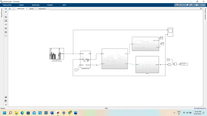
The model has four subsystems which are explained one by one in each block

1. vehicle body subsystem

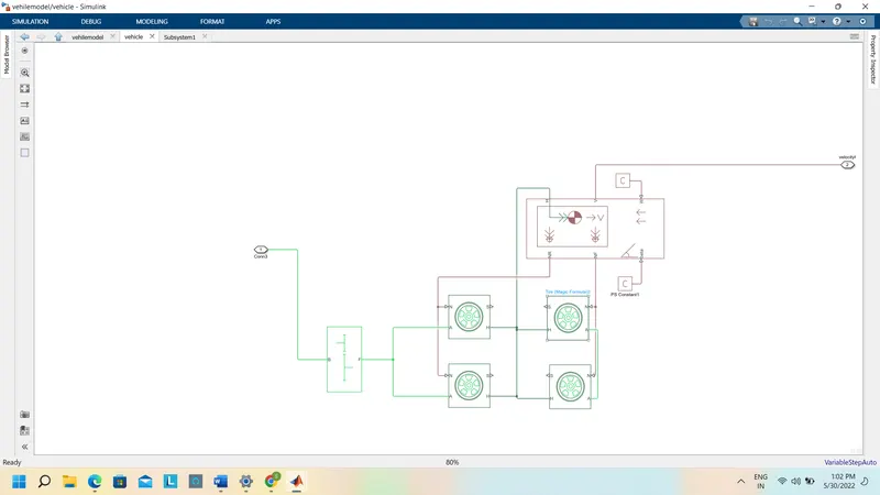
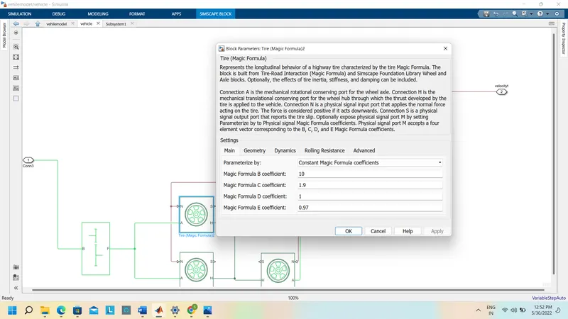
A) Tire (Magic Formula)

A tire with longitudinal behavior given by Magic Formula coefficients

expand all on page

Library:
Simscape / Driveline / Tires & Vehicles

Description

The Tire (Magic Formula) block models a tire with longitudinal behavior given by the Magic Formula [1], an empirical equation based on four fitting coefficients. The block can model tire dynamics under constant or variable pavement conditions.

The longitudinal direction of the tire is the same as its direction of motion as it rolls on the pavement. This block is a structural component based on the Tire-Road Interaction (Magic Formula) block.

To increase the fidelity of the tire model, you can specify properties such as tire compliance, inertia, and rolling resistance. However, these properties increase the complexity of the tire model and can slow down the simulation. Consider ignoring tire compliance and inertia if simulating the model in real-time or if preparing the model for hardware-in-the-loop (HIL) simulation.

Tire Model

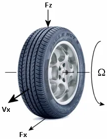
The Tire (Magic Formula) block models the tire as a rigid wheel-tire combination in contact with the road and subject to slip. When torque is applied to the wheel axle, the tire pushes on the ground (while subject to contact friction) and transfers the resulting reaction as a force back on the wheel. This action pushes the wheel forward or backward. If you include the optional tire compliance, the tire also flexibly deforms under load.

The figure shows the forces acting on the tire. The table defines the tire model variables.

B) the vehicle body

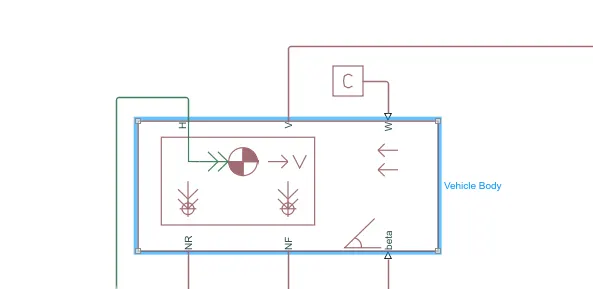
This section is intended to give guidance on the design of chassis for electric vehicles. Chassis design should be carried out in conjunction with other texts on chassis design, not to mention computer packages that specialize in this area. Nevertheless, a basic understanding of what the chassis should do and other parameters related to electric vehicle chassis is needed.

In the early cars, chassis and bodies were separate items. The chassis gave the basic strength of the vehicle while the body and glazing acted as a cocoon to keep the passengers and luggage protected from the outside elements.

In recent times the body and chassis have been combined as a monocoque so that every part, including the glazing, adds to the strength and stiffness, resulting in a much lighter vehicle. Either monocoques or separate chassis/body units are an acceptable basis for design. Despite the popularity of monocoques, several modern electric vehicles use a separate chassis, most notably the advanced new General Motors Hy-wire fuel cell vehicle, which will be discussed in more detail later.

It is worth pausing to think precisely what the chassis/body does; ideally, a chassis/body should fill the following criteria. It should:

• not vibrate, particularly at frequencies and harmonics of rotating parts;

• be aerodynamic;

• be resistant to impact;

• crumple evenly in an accident, minimizing forces on driver/passengers;

• be strong enough to fix components easily;

• be impact and roll resistant;

• be aesthetically pleasing;

• be corrosion-proof.

Chassis/body design requires optimization of conflicting requirements such as cost and strength, or performance and energy efficiency. There are important differences when designing electric vehicles compared to their IC equivalents. For example, extra weight is not so important with an internal combustion vehicle, were a little more power can be cheaply added to compensate for a slightly heavier chassis. The same is true for aerodynamic drag, where a slight increase in drag can be similarly compensated for. Savings in weight, as well as increases in efficiency, contribute directly to the size of the batteries, and these, are both heavy and expensive.

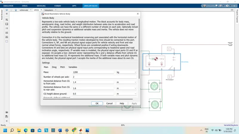
Simple Gear

Simple gear of base and follower wheels with adjustable gear ratio, friction losses, and triggered faults

expand all on page

Library:
Simscape / Driveline / Gears

Description

The Simple Gear block represents a gearbox that constrains the connected driveline axes of the base gear, B, and the follower gear, F, to corotate with a fixed ratio that you specify. You choose whether the follower axis rotates in the same or opposite direction as the base axis. If they rotate in the same direction, the angular velocity of the follower, ω_F, and the angular velocity of the base, ω_B, have the same sign. If they rotate in opposite directions, ω_F and ω_B have opposite signs.

Ideal Gear Constraint and Gear Ratio

The kinematic constraint that the Simple Gear block imposes on the two connected axes is

rFωF=rBωB

where:

r_F is the radius of the follower gear.
ω_F is the angular velocity of the follower gear.
RB_B is the radius of the base gear.
ω_B is the angular velocity of the base gear.

The follower-base gear ratio is

gFB=rFrB=NFNB

where:

N_B is the number of teeth in the base gear.
N_BF is the number of teeth in the follower gear.

Reducing the two degrees of freedom to one independent degree of freedom yields the torque transfer equation

gFBτB+τF−τloss=0

where:

τ_B is the input torque.
τ_F is the output torque.
τ_loss is the torque loss due to friction.

For the ideal case, τloss=0.

Nonideal Gear Constraint and Losses

In the nonideal case, τloss≠0. For general considerations on nonideal gear modeling, see Model Gears with Losses.

In a nonideal gear pair (B, F), the angular velocity, gear radii, and gear teeth constraints are unchanged. But the transferred torque and power are reduced by:

Coulomb friction between teeth surfaces on gears B and F, characterized by efficiency, η
Viscous coupling of driveshafts with bearings, parametrized by viscous friction coefficients, μ

Constant Efficiency

In the constant efficiency case, η is constant, independent of load or power transferred.

Load-Dependent Efficiency

In the load-dependent efficiency case, η depends on the load or power transferred across the gears. For either power flow,

τCoul=gFBτidle+kτF

where:

τ_Coul is the Coulomb friction-dependent torque.
k is a proportionality constant.
τ_idle is the net torque acting on the input shaft in idle mode.

Efficiency, η, is related to τ_Coul in the standard, preceding form but becomes dependent on load:

η=τFgFBτidle+(k+1)τF

Faults

If you enable faults for the block, the efficiency changes in response to one or both of these triggers:

Simulation time — A fault occurs at a specified time.
Simulation behavior — A fault occurs in response to an external trigger. Enabling an external fault trigger exposes port, T.

If a fault trigger occurs, for the remainder of the simulation, the block uses the faulted efficiency in one of these ways:

Throughout rotation
When the rotation angle is within a faulted range that you specify

You can program the block to issue a fault report as a warning or error message.

Thermal Model

You can model the effects of heat flow and temperature change by enabling the optional thermal port. To enable the port, set the Friction model to Temperature-dependent efficiency.

Additionally, you can choose to model efficiency that varies with loading and temperature by setting the Friction model to Temperature and load-dependent efficiency. Selecting a thermal variant:

Exposes port H, a conserving port in the thermal domain.
Enables the Thermal mass parameter, which allows you to specify the ability of the component to resist temperature changes.
Enables the Initial Temperature parameter, which allows you to set the initial temperature.

2. power controller subsystem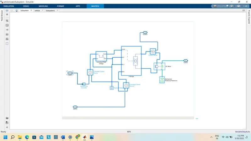

A.Dc motor:-

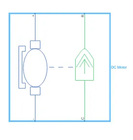
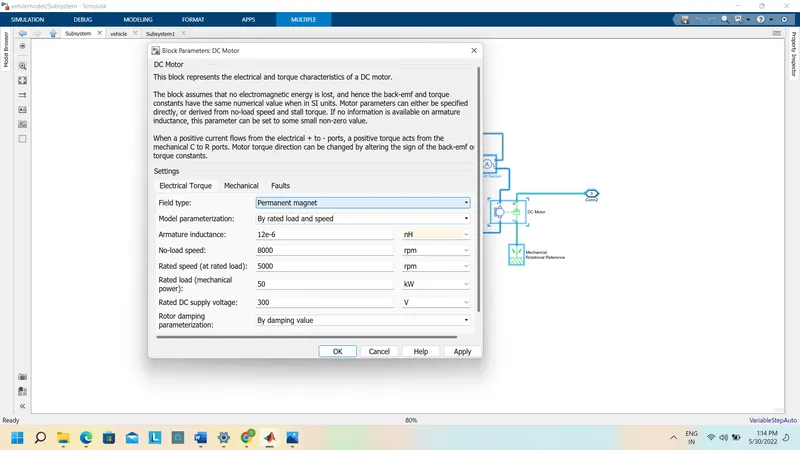
The output is the speed of the motor, calculated by multiplying the value from the input port by the value of the Gearing Ratio parameter and rounding the product to the nearest integer. Connect a Sink block, such as a Display block or Scope block, to the output port to view the simulation output.

the parameter change in this block are

No_load speed =6000rpm

rated speed at rated load is 4000 rpm

Rated load (mech power)=5000w

the rated Dc supply vtg 1.5v
The remaining is to keep constant

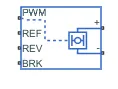
H-Bridge

H-bridge motor driver

expand all on page

Library:
Simscape / Electrical / Semiconductors & Converters / Converters

Description

The H-Bridge block represents an H-bridge motor driver. The block has the following two Simulation mode options:

PWM — The H-Bridge block output is a controlled voltage that depends on the input signal at the PWM port. If the input signal has a value greater than the Enable threshold voltage parameter value, the H-Bridge block output is on and has a value equal to the value of the Output voltage amplitude parameter. If it has a value less than the Enable threshold voltage parameter value, the block maintains the load circuit using one of the following three Freewheeling mode options:
- Via one semiconductor switch and one freewheeling diode
- Via two freewheeling diodes
- Via two semiconductor switches and one freewheeling diode
The first and third options are sometimes referred to as an asynchronous operations.

The signal at the REV port determines the polarity of the output. If the value of the signal at the REV port is less than the value of the Reverse threshold voltage parameter, the output has positive polarity; otherwise, it has negative polarity.
Averaged — This mode has two Load current characteristics options:
- Smoothed
- Unsmoothed or discontinuous
The Smoothed option assumes that the current is practically continuous due to load inductance. In this case, the H-Bridge block output is:

VOVPWMAPWM−IOUTRON

where:
- V_O is the value of the Output voltage amplitude parameter.
- V_PWM is the value of the voltage at the PWM port.
- A_PWM is the value of the PWM signal amplitude parameter.
- I_OUT is the value of the output current.
- R_ON is the Bridge on the resistance parameter.
The current will be smooth if the PWM frequency is large enough. Synchronous operation where freewheeling is via a bridge arm back to the supply also helps smooth the current. For cases where the current is not smooth, or possibly discontinuous (that is, it goes to zero between PWM cycles), use the Unsmoothed or discontinuous option. For this option, you must also provide values for the Total load series resistance, Total load series inductance, and PWM frequency. During simulation, the block uses these values to calculate a more accurate value for H-bridge output voltage that achieves the same average current as would be present if simulating in PWM mode.

Set the Simulation mode parameter to Averaged to speed up simulations when driving the H-Bridge block with a Controlled PWM Voltage block. You must also set the Simulation mode parameter of the Controlled PWM Voltage block to Averaged mode. This applies the average of the demanded PWM voltage to the motor. The accuracy of the Averaged mode simulation results relies on the validity of your assumption about the load current. If you specify that the current is Unsmoothed or discontinuous, then the accuracy also depends on the values you provide for load resistance and inductance being representative. This mode also makes some simplifying assumptions about the underlying equations for the case when the current is discontinuous. For typical motor and bridge parameters, accuracy should be within a few percent. To verify Averaged mode accuracy, run the simulation using the PWM mode and compare the results to those obtained from using the Averaged mode.

Braking mode is invoked when the voltage presented at the BRK port is larger than the Braking threshold voltage. Regardless of whether in PWM or Averaged mode, when in braking mode the H-bridge is modeled by a series combination of two resistances R1 and R2 where:

R1 is the resistance of a single bridge arm, that is, half the value of the Total bridge on the resistance parameter.
R2 is the resistance of a single bridge arm in parallel with a diode resistance, that is, R1 · Rd / ( R1 + Rd ), where Rd is the diode resistance.

External Power Supply

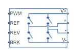
To model the demands placed on the DC supply, you can choose to expose the power supply ports of the H-Bridge block by setting the Power supply parameter to External. If the power supply ports are exposed, then only PWM simulation mode is supported.

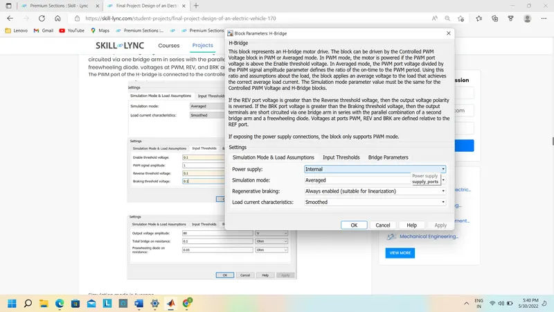
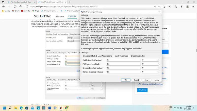
The simulation model is avg

Enabled threshold Voltage is 0.1v

PWM signal amplitude is 1v

reverse threshold voltage is 0.1v

braking threshold voltage is 0.1v

output vtg amplitude is 80v

Controlled PWM Voltage

Pulse-width modulated voltage source

expand all on page

Library:
Simscape / Electrical / Integrated Circuits

Description

The Controlled PWM Voltage block represents a pulse-width modulated (PWM) voltage source. The block has two modeling variants, accessible by right-clicking the block in your block diagram and then selecting the appropriate option from the context menu, under Simscape > Block choices:

Electrical input ports — The block calculates the duty cycle based on the reference voltage across its ref+ and ref- ports. This modeling variant is the default.
PS input — Specify the duty cycle value directly by using an input physical signal port.

For the Electrical input ports variant of the block, the demanded duty cycle is

100∗Vref−VminVmax−Vmin percent

where:

V_ref is the reference voltage across the ref+ and ref- ports.
V_min is the minimum reference voltage.
V_max is the maximum reference voltage.
the parameter change in this block are

Simulation mode is avrge=

input vtg for 100% duty cycle is 1

output vtg amp is 1

The remaining is to keep constant

battery subsystem:-

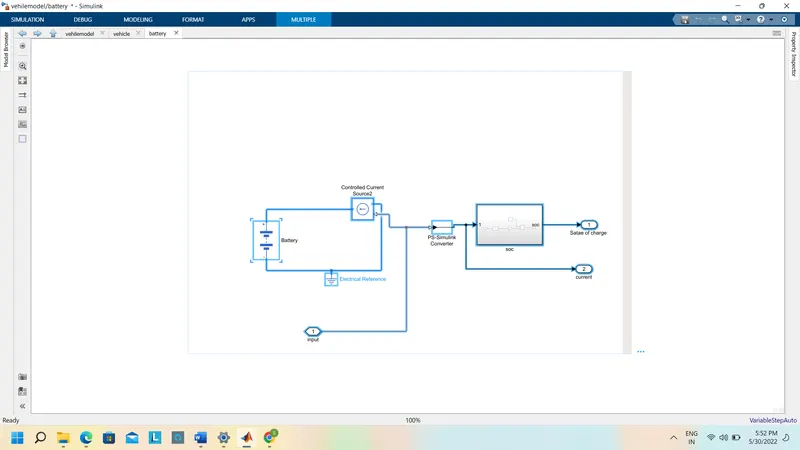
Soc( state of charge )

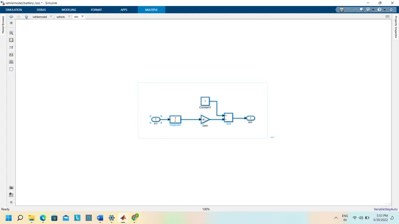
A) Battery

Behavioral battery model

expand all on page

Library:
Simscape / Electrical / Sources

Description

The Battery block represents a simple battery model. The block has four modeling variants, accessible by right-clicking the block in your block diagram and then selecting the appropriate option from the context menu, under Simscape > Block choices:

Uninstrumented | No thermal port — A basic model that does not output battery charge level or simulates thermal effects. This modeling variant is the default.
Uninstrumented | Show thermal port — Model with exposed thermal port. This model does not measure the internal charge level of the battery.
Instrumented | No thermal port — Model with an exposed charge output port. This model does not simulate thermal effects.
Instrumented | Show thermal port — Model that lets you measure the internal charge level of the battery and simulate thermal effects. Both the thermal port and the charge output port are exposed.

The instrumented variants have an extra physical signal port that outputs the internal state of charge. Use this functionality to change load behavior as a function of the state of charge, without the complexity of building a charge state estimator.

The thermal port variants expose a thermal port, which represents the battery's thermal mass. When you select this option, provide additional parameters to define battery behavior at a second temperature. For more information, see Modeling Thermal Effects.

The battery equivalent circuit is made up of the fundamental battery model, the self-discharge resistance R_SD, the charge dynamics model, and the series resistance R₀.

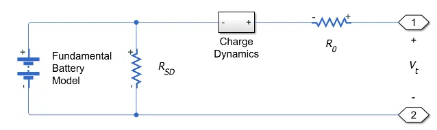
Battery Model

If you select Infinite for the Battery charge capacity parameter, the block models the battery as a series resistor and a constant voltage source. If you select Finite for the Battery charge capacity parameter, the block models the battery as a series resistor and a charge-dependent voltage source. In the finite case, the voltage is a function of charge and has the following relationship:

V=V0(SOC1−β(1−SOC))

where:

SOC (state-of-charge) is the ratio of current charge to-rated battery capacity.
V₀ is the voltage when the battery is fully charged at no load, as defined by the Nominal voltage, the Vnom parameter.
β is a constant that is calculated so that the battery voltage is V1 when the charge is AH1. Specify the voltage V1 and ampere-hour rating AH1 using block parameters. AH1 is the charge when the no-load (open-circuit) voltage is V1, and V1 is less than the nominal voltage.

The equation defines an approximate relationship between voltage and remaining charge. This approximation replicates the increasing rate of voltage drop at low charge values and ensures that the battery voltage becomes zero when the charge level is zero. The advantage of this model is that it requires few parameters, which are readily available on most datasheets.

Modeling Battery Fade

For battery models with finite battery charge capacity, you can model battery performance deterioration depending on the number of discharge cycles. This deterioration is referred to as battery fade. To enable battery fade, set the Battery fade parameter to Enabled. This setting exposes additional parameters in the Fade section.

The block implements battery fade by scaling certain battery parameter values that you specify in the Main section, depending on the number of completed discharge cycles. The block uses multipliers λ_AH, λ_R0, and λ_V1 on the Ampere-hour rating, Internal resistance, and Voltage V1 when the charge is AH1 parameter values, respectively. These multipliers, in turn, depend on the number of discharge cycles:

λAH=1−k1N0.5

λR0=1+k2N0.5

λV1=1−k3N

N=N0+1AHt0i(t)⋅H(i(t))λAH(t)dt

where:

λ_AH is the multiplier for battery nominal capacity.
λ_R0 is the multiplier for battery series resistance.
λ_V1 is the multiplier for voltage V1.
N is the number of discharge cycles completed.
N₀ is the number of full discharge cycles completed before the start of the simulation.
AH is the rated battery capacity in ampere-hours.
i(t) is the instantaneous battery output current.
H(i(t)) is the Heaviside function of the instantaneous battery output current. This function returns 0 if the argument is negative, and 1 if the argument is positive.

The block calculates the coefficients k₁, k₂, and k₃ by substituting the parameter values you provide in the Fade section into these battery equations. For example, the default set of block parameters corresponds to the following coefficient values:

k₁ = 1e-2
k₂ = 1e-3
k₃ = 1e-3

You can also define a starting point for a simulation based on the previous charge-discharge history by using the high-priority variable Discharge cycles. For more information, see Variables.

Modeling Thermal Effects

For thermal variants of the block, you provide additional parameters to define battery behavior at a second temperature. The extended equations for the voltage when the thermal port is exposed are:

V=V0T(SOC1−βT(1−SOC))

V0T=V0(1+λV(T−T1))

where:

T is the battery temperature.
T₁ is the nominal measurement temperature.
λ_V is the parameter temperature dependence coefficient for V₀.
βT=β[1+λβ(T−T1)].
λ_β is the parameter temperature dependence coefficient for β.
β is calculated in the same way as Battery Model, using the temperature-modified nominal voltage V_0T.

The internal series resistance, self-discharge resistance, and any charge-dynamic resistances are also functions of temperature:

RT=R(1+λR(T−T1))

where λ_R is the parameter temperature dependence coefficient.

All the temperature dependence coefficients are determined from the corresponding values you provide at the nominal and second measurement temperatures. If you include charge dynamics in the model, the time constants vary with temperature in the same way.

The battery temperature is determined from a summation of all the ohmic losses included in the model:

Mth˙T=iVT,i2/RT,i

where:

M_th is the battery thermal mass.
I correspond to the ith ohmic loss contributor. Depending on how you have configured the block, the losses include:
- Series resistance
- Self-discharge resistance
- First charge dynamics segment
- Second charge dynamics segment
- Third charge dynamics segment
- Fourth charge dynamics segment
- Fifth charge dynamics segment
V_{T, i} is the voltage drop across resistor i.
R_{T, i} is resistor i.

Drive cycle source

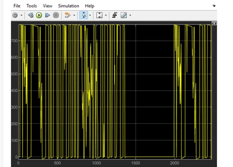
Standard or specified longitudinal drive cycle

Library:
Powertrain Blockset / Vehicle Scenario Builder

Vehicle Dynamics Blockset / Vehicle Scenarios / Drive Cycle and Maneuvers

Description

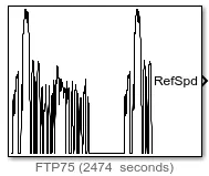
The Drive Cycle Source block generates a standard or user-specified longitudinal drive cycle. The block output is the specified vehicle longitudinal speed, which you can use to:

Predict the engine torque and fuel consumption that a vehicle requires to achieve desired speed and acceleration for a given gear shift reference.
Produce realistic velocity and shift references for closed-loop acceleration and braking commands for vehicle control and plant models.
Study, tune, and optimize vehicle control, system performance, and system robustness over multiple drive cycles.
Identify the faults within tolerances specified by standardized tests, including:
- EPA dynamometer driving schedules¹
- Worldwide Harmonised Light Vehicle Test Procedure (WLTP) laboratory tests²

For the drive cycles, you can use:

Drive cycles from predefined sources. By default, the block includes the FTP–75 drive cycle. To install additional drive cycles from a support package, see Install Drive Cycle Data. The support package has drive cycles that include the gear shift schedules, for example, JC08 and CUEDC.
Workspace variables that define your drive cycles.
.mat, .xls, .xlsx, or .txt files.
worldwide-open bottle (WOT) parameters, including initial and nominal reference speed, deceleration start time, and final reference speed.

Longitudinal Driver

Longitudinal speed-tracking controller

expand all on page

Library:
Powertrain Blockset / Vehicle Scenario Builder

Vehicle Dynamics Blockset / Vehicle Scenarios / Driver

Description

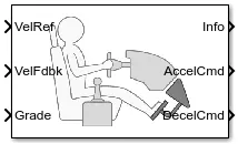
The Longitudinal Driver block implements a longitudinal speed-tracking controller. Based on reference and feedback velocities, the block generates normalized acceleration and braking commands that can vary from 0 through 1. You can use the block to model the dynamic response of a driver or to generate the commands necessary to track a longitudinal drive cycle.

Configurations

External Actions

Use the External Actions parameters to create input ports for signals that can disable, hold, or override the closed-loop acceleration or deceleration commands. The block uses this priority order for the input commands: disable (highest), hold, override.

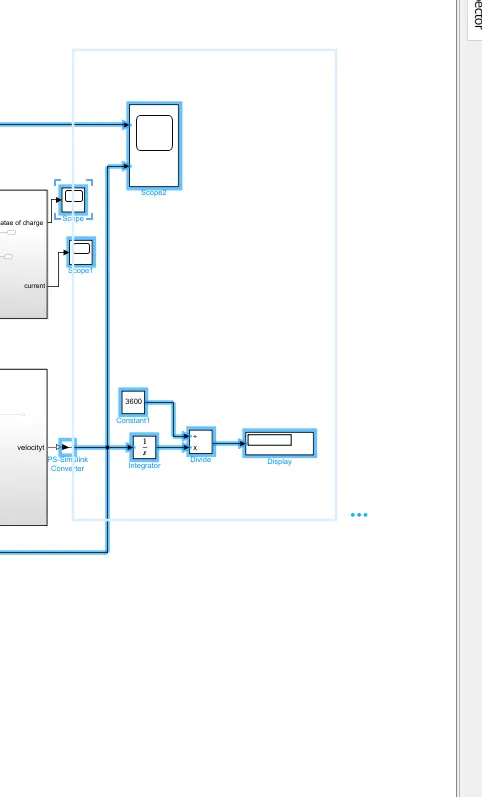
SUBSYSTEM ODF DISTANCE CALCULATION

RESULT:-

So at the end of the FTP75 drive cycle ,the total distance Ttraveledby the vehicle is 22km

A.drive cycle

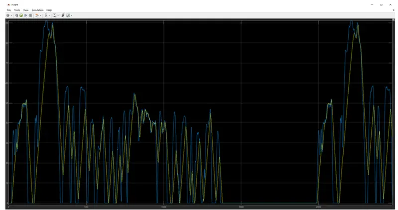
Plot of current

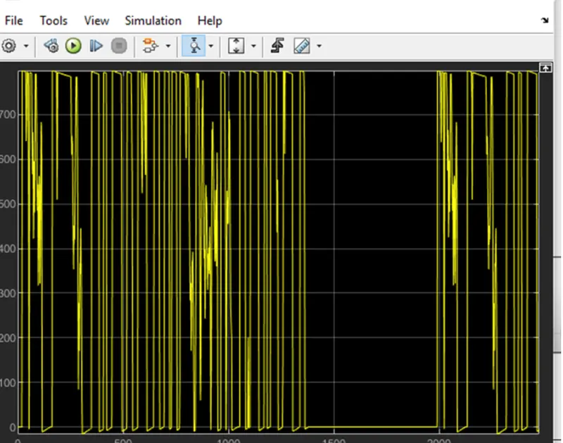
Battery current plot

Final Project: Design of an Electric Vehicle