Final Project: Design of an Electric Vehicle
Create a MATLAB model of electric car which uses a battery and a DC motor. Choose suitable blocks from Powertrain block set. Prepare a report about your model including following:
Objectives:
1. System level configurations
2. Model parameters
3. Results
4. Conclusion
Software Used:
MATLAB R-2021a Simulink.
Block Diagram of EV:
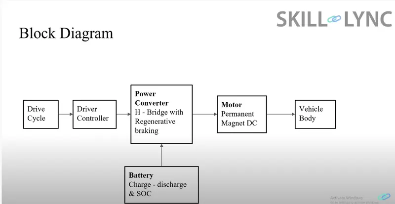
In the Designed EV main blocks are DC motor, Battery, H-Bridge, drive cycle, PWM controller, longitudinal driver, vehicle body and transmission system. Drive cycle is a input data like a human drive his actual vehicle is FTP75 drive cycle is introduced to make a designed vehicle to give the output how it reacts to the drive cycle. The main object is spped by driver to estimate the state of charge (SOC) and distance travelled by the vehicle.
Simulink Model of Electric Vehicle (car):
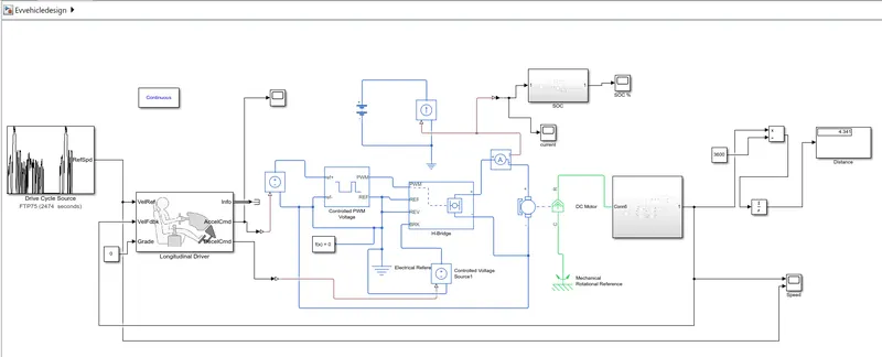
In this the current flows to the DC motor from the battery through DC-DC power converter to drive the motor. The required voltage will be controlled in the controlled PWM votage. The controller will follow the given drive cycle and run the motor in the rpm. The motor power is transmitted to the wheels of a vehicle through the gear box.
Model parameters:
Vehicle Body Subsystem:
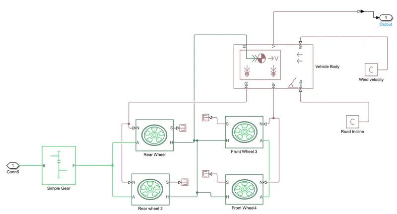
In this vehicle body we have used four tyres, simple gear, vehicle body. This is the Rear wheel drive. The connections of body to tyres is to connect the HUB first to all four tyres. The NF and NR is the physical output ports which is the front and rear normal wheel force.
In this motor will produce the rotational output which will give the velocity body and transmission system. The rotational output is taken by the gear system here to maintain the constant speed through out the transmission without any loss in speed from the motor to tyres. The above diagram is the subsystem of ev vehicle model. The gear output is given to axel of rear wheels because it is a rear wheel drive.
Vehicle Body:
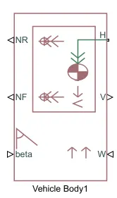
In the above figure the H is the HUB, NR - normal force of rear wheel and NF - normal force of front wheel and where V is the Velocity which is given to the output.
The W is the Wind velocity the value is given to this is 0 and its parameter in m/s.
The BETA is the Road incline in this also the value is 0 and its parameter is in rad.
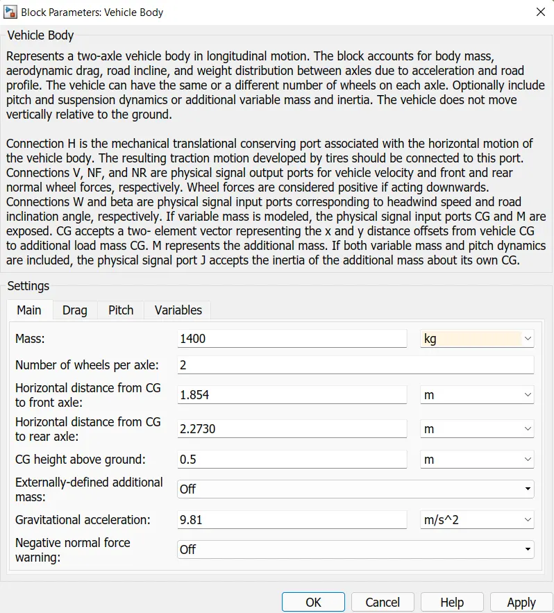
The above figure shows the vehicle body parameters which i given the mass is 1400 kg and no.of wheels per axle is 2 and remaining values is given as default.
Wheel:
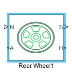
The tyre is shown above fig. In this the N is physical output port that applies the normal force acting on tyre. The N port is connecting to the NR/NF to vehicle body. The Axel is connecting to the simple gear for the transmission. The S is the slip.
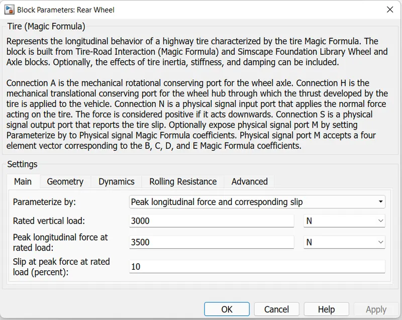
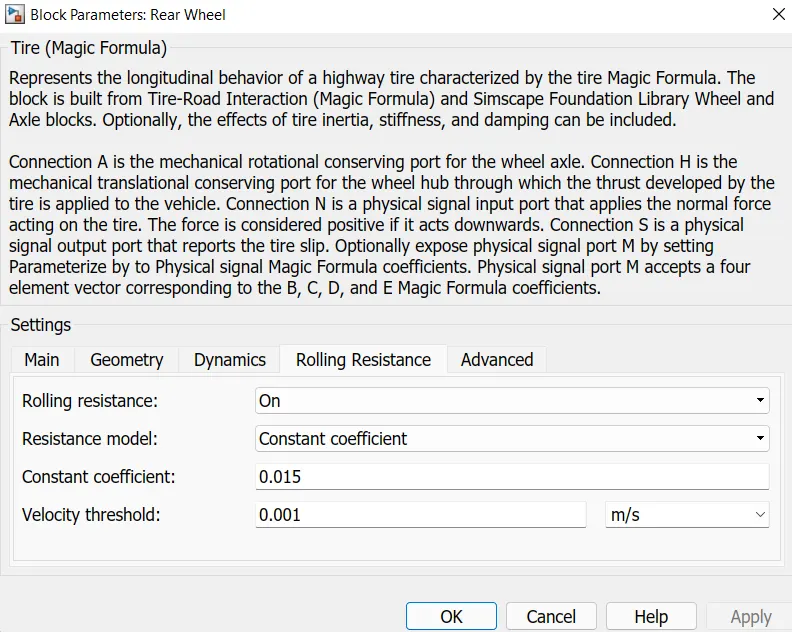
The Wheel block parameters is "peak longitudinal force and corresponding slip" and the rolling resistance parameters is set by as default.
Simple Gear:
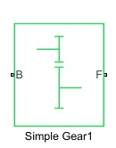
The simple gear block represents fixed-ratio gear. It has two terminals B and F. The B represents the Base and the F is the Follower. The B is connected to the motor to get the power and the F is connected to the Axel of the vehicle.
In this the parameter is set as default.
Motor and Control System:
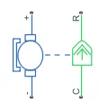
DC Motor
The block represents electrical and torque characteristics of a DC motor.
The block assumes no electromagnetic energy is lost, and hence back emf and torque constants have the same numerical value when in SI units.
The positive terminal + , - is the electrical connections is that controllers. And the R, C is the mechanical ports which is C connects to the mechanical rotational reference and R is connected to the Simple gear of the vehicle body.
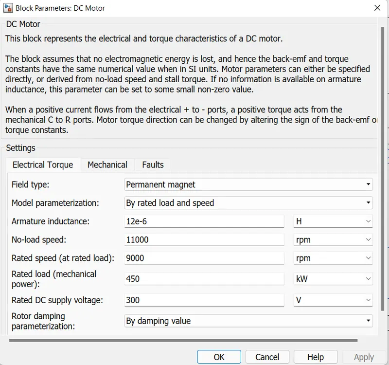
The above fig shows the DC motor parameters which i given the DC supply voltage is 300 and the no-load speed is 11000 Rated speed = 9000, Rated load = 450. This is set to be Rated load and speed.
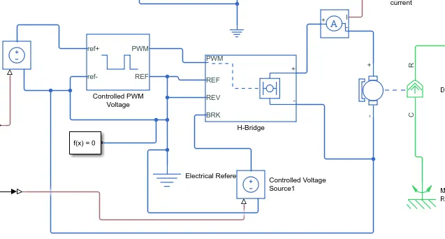
The above fig shows the controller which is connected the H-Bridge, Controlled PWM voltage, Slover configuration, current sensor, electrical reference, controlled voltage source. The controlled PWM voltage is connected to the longitudinal driver through controlled voltage source.
The H-bridge +,- is connected to the dc motor through current sensor. The PWM is connected to PWM of controlled PWM voltage and REF to REF and both REF is connected to the Electrical reference. All these components are the simscape electrical components so they need solver configuration block which helps to slove the simulation. The BRK is given to controlled voltage source and that to longitudinal driver brake.
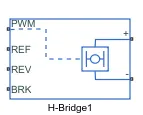
H-BRidge
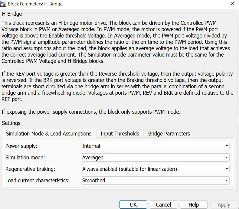
The block parameters are power supply is in internal because it is a motor controller that has IGBT components aligned in the shade of H and eill operate only two at a time to the input signal from PWM block. The simulation mode is averaged and the regenerative braking is always enable. THe load current is smoothed.
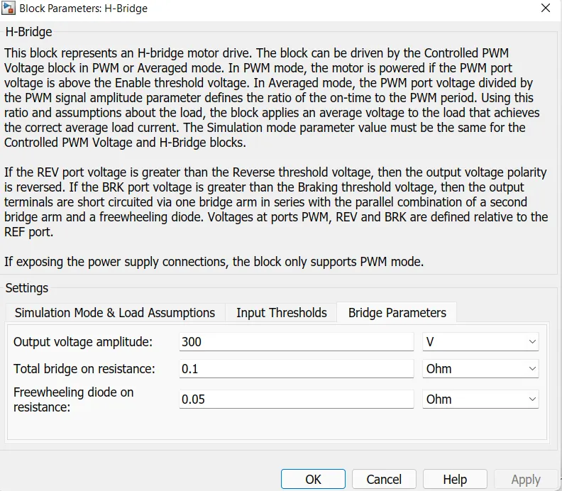
The Bridge parameters are output voltage amplitude is 300 i given and the input thresholds are set as default.
Controlled PWM Voltage:
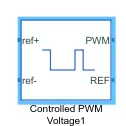
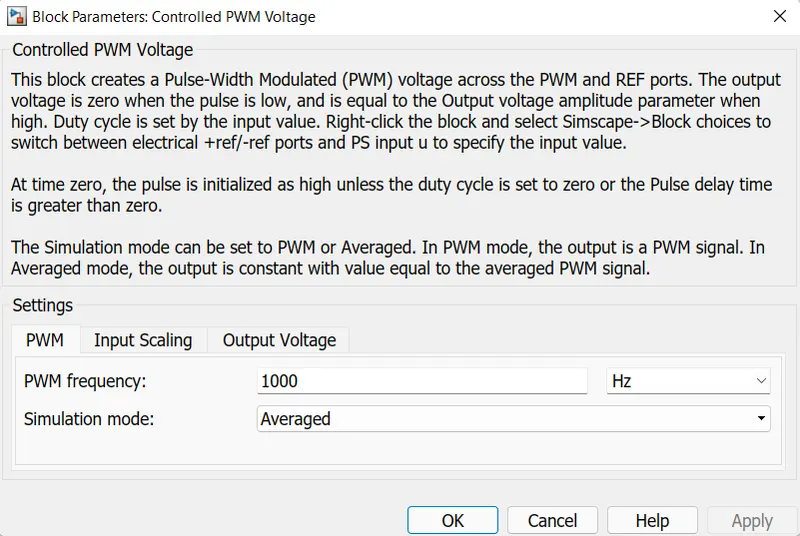
IN this the PWM is connected to the PWM of H-bridge. THE ref+ and ref- ports are given controlled voltage source. The PWM frequency is 1000 hz and simulation mode is Averaged is set as default. The output vltage is 300.
Battery:

This block models a battery. If you select Infinite for the Battery charge capacity parameter, the block models the battery as a series internal resistance and a constant voltage source. If you select Finite for the Battery charge capacity parameter, the block models the battery as a series internal resistance plus a charge-dependent voltage source defined by:
V = Vnom*SOC/(1-beta*(1-SOC))
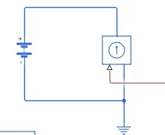
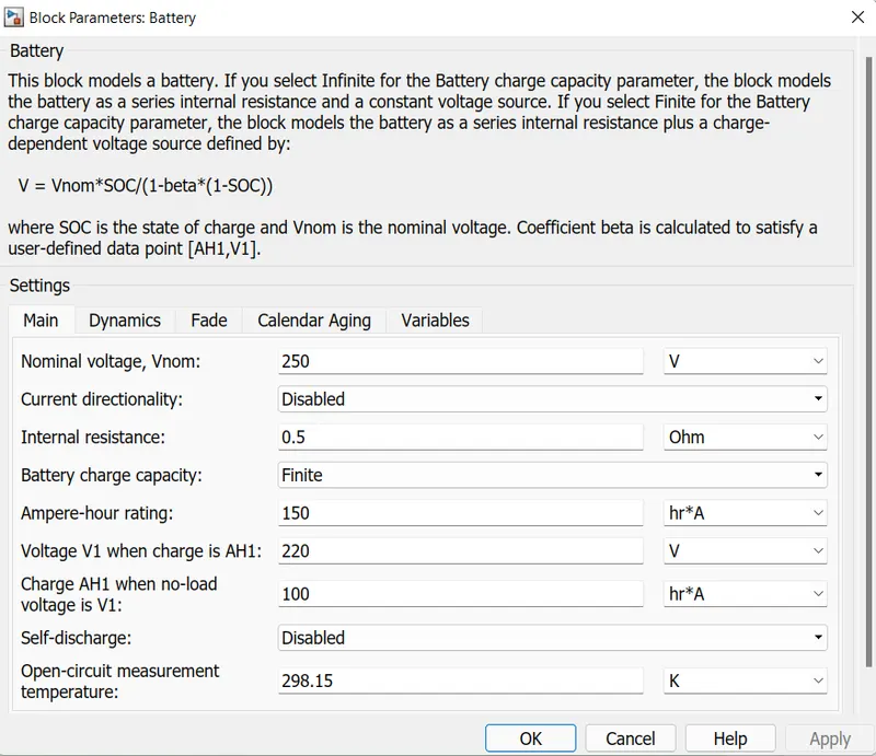
In this the nominal voltage is 250 v, Internal resistance is 0.5 ohm, Ampere hour rating is 150, voltage v1 is 220 v is to applied.
Estimate SOC:
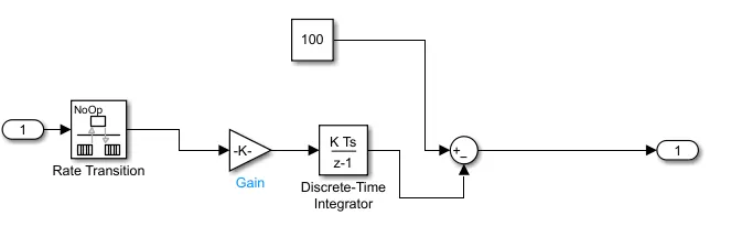
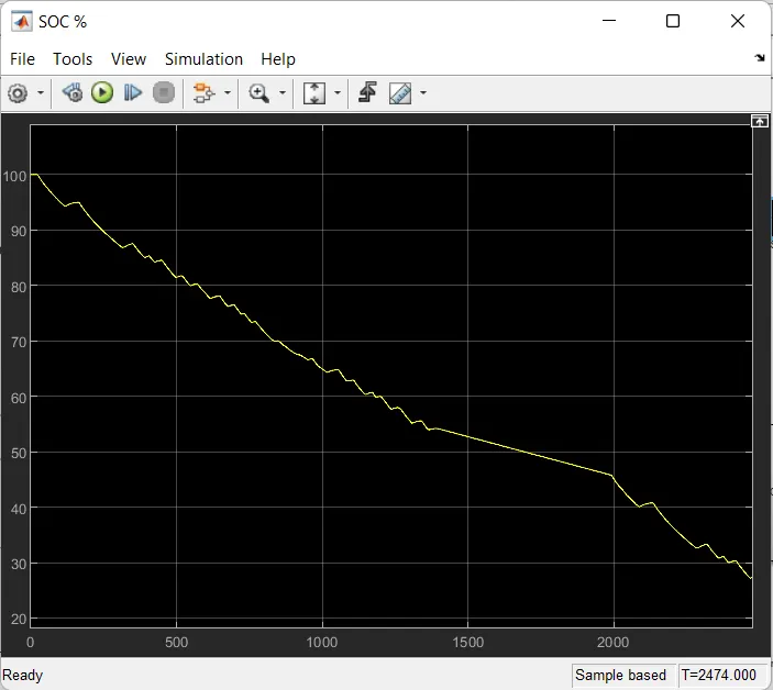
State of charge is percentage or level of battery presents after certain travel or consumption of battery charge by the vehicle. In designed vehicle SOC is calculated by the given it to the rate transition and then to gain then to discrete-time integrator and it will get minus from the 1 as it is considered a 100% of battery.
Drive Cycle:
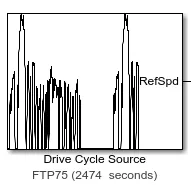
Generates a standard or user-specified longitudinal drive cycle. The block output is the vehicle longitudinal speed. You can import drive cycles from:
1.Predefined sources
2. Workspace variables, including arrays and time series objects
The drive cycle is in FTP75 (2474 seconds). This drive cycles are standard drive cycle which is used to test the vehicle performance.
Longitudinal Driver:
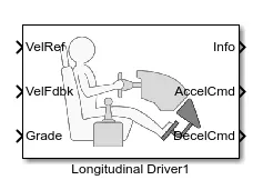
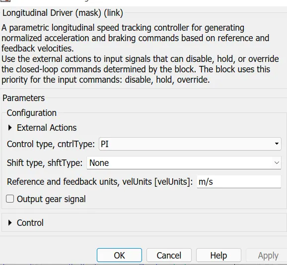
The Longitudinal Driver block implements a longitudinal speed-tracking controller. Based on reference and feedback velocities, the block generates normalized acceleration and braking commands that can vary from 0 through 1. You can use the block to model the dynamic response of a driver or to generate the commands necessary to track a longitudinal drive cycle.
Proportional-integral (PI) control with tracking windup and feed-forward gains.
PI control with tracking windup and feed-forward gains that are a function of vehicle velocity.
Result:
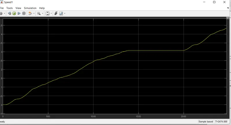
Distance Plot:
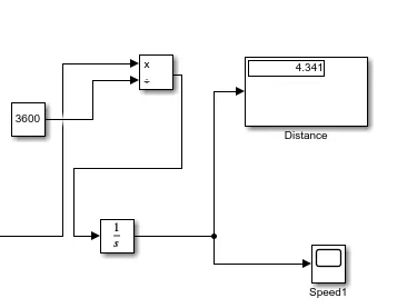
The end of the result is FTP75 drive cycle, the total distance travelled by the vehicle is 4.341 KM.
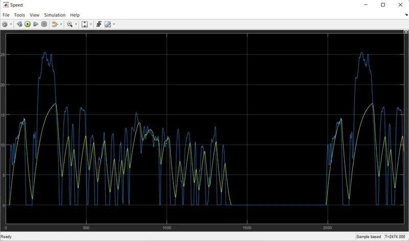
Speed Plot: The speed graph is shown in yellow colour line which travelled and blue line shows the actual drive cycle.
SOC: The state of charge represents the battery capacity left for the vehicle and it is showed by the below graph.
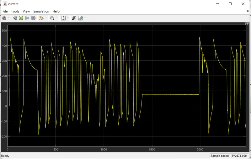
Current Plot: During simulations is almost constant at high speeds and high amounts of currents are taken by the motor.
Conclusion:
The Electric vehicle matlab model is created according to FTP75 drive cycle and it travels 4.3 km.