Final Project: Design of an Electric Vehicle
Design of an electric vehicle
Aim:
To create a MATLAB model of an electric car that uses a DC motor, Vehicle body, Battery, and suitable blocks from the powertrain blockset.
Objectives:
An electric vehicle (EV) is an automotive vehicle that uses one or more electric motors for propulsion. It is eco-friendly and has higher efficiency. The batteries used in the system are recharged using AC/DC charging technologies. AC charging is slow when compared to DC charging.
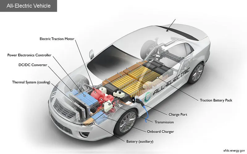
The above picture shows the pictorial representation of an electric vehicle. The electrical vehicle has a Power electronic controller for controlling the operation of the vehicle. DC-DC converter, cooling system, and battery are major parts of the vehicle.
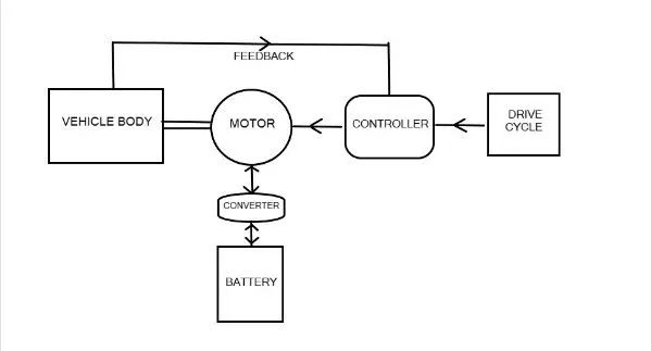
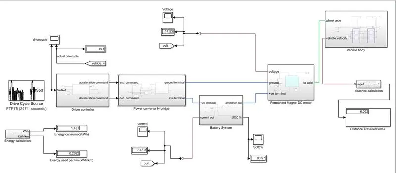
In the system model, the Drive cycle is given as an input. The input is connected with a controller in which a controlled voltage source, controlled PWM voltage, and H-Bridge are used for the operation. The controller is connected to a DC motor, where a voltage sensor is used for measuring the voltage. As same, the controller battery and the vehicle body are connected with a motor.
Simulink Model:
Drive Cycle:
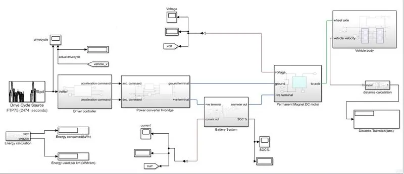
The drive cycle source block is used as an input for the Simulink model. In that drive cycle, I am choosing
'FTP75' is a predefined drive cycle with a duration of 2474 seconds.
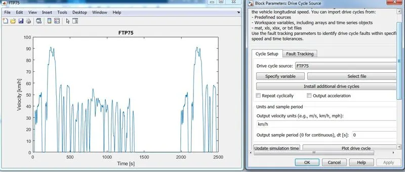
The above plot diagram shows the predefined input values of an 'FTP75' drive cycle block. The reference speed of the input block is connected with the drive controller and the output values of the drive cycle are expressed through the scope.
Driver Controller:
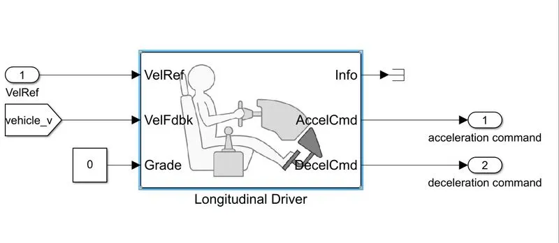
A parametric longitudinal speed tracking controller for both generating normalized acceleration and braking commands is based on velocity reference and velocity feedback. Here the terminator block is used to terminate the output signals for preventing the model from the warning of unconnected output ports.
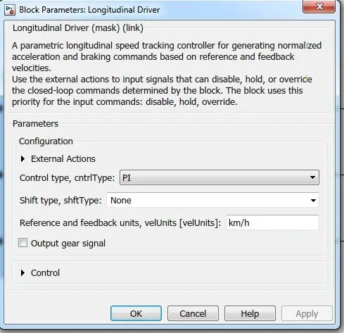
The driver gives the acceleration and deceleration commands according to the drive cycle data and it gives the acceleration and deceleration commands to the power converter block. Here we are obtaining gradeability through the constant block.
Power Converter:
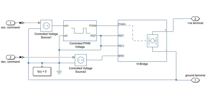
In this block, the acceleration and deceleration commands are given to both controlled voltage sources from the driver controller. The controlled voltage from the acceleration command is given as the reference voltage to the controlled PWM voltage.
1. Controlled Voltage Source:
The block represents an ideal voltage source that is powerful enough to maintain the specified voltage at its output regardless of the current passing through it. The output voltage is V = Vs, where Vs is the numerical value presented at the physical signal port.
Here the acceleration and deceleration commands are given to both controlled voltage sources from the driver controller.
2. Controlled PWM Voltage: This block creates a Pulse-Width Modulated voltage across the PWM and REF ports. when the pulse is high, the output voltage is equal to the amplitude parameter and the pulse is low when the output voltage is zero.
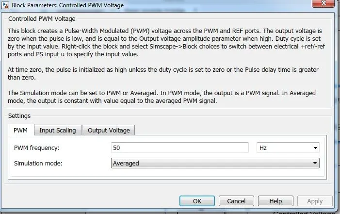
At the time zero, the pulse is initialized as high. Unless the duty cycle is set to zero or the pulse delay time is greater than zero. The simulation mode can be set to PWM or Averaged. In PWM mode the output will be a PWM signal and In the average mode, the output is constant with a value equal to the averaged PWM signal. Here I am using averaged simulation mode for the operation.
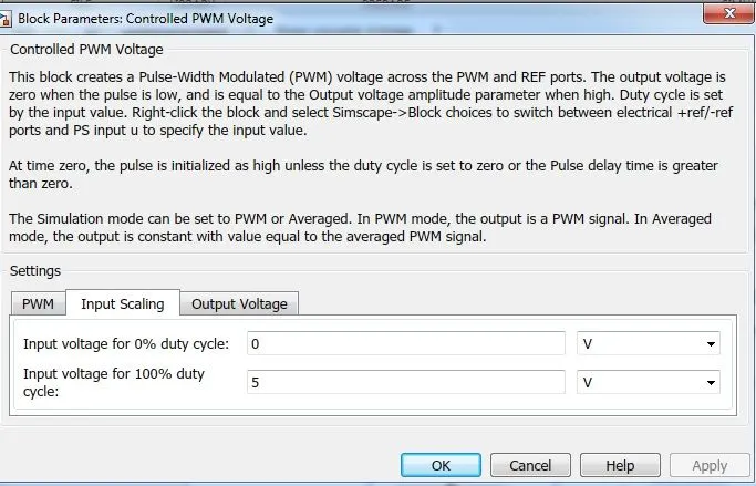
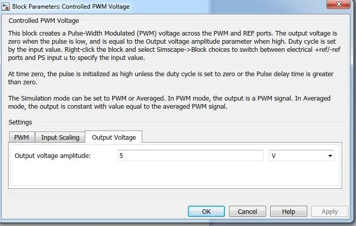
The reference voltage of controlled PWM voltage is connected with REV terminal of H-Bridge for regenerative braking and the brake input of H-Bridge is connected with controlled PWM voltage which receives the deceleration command.
3. H-Bridge:
This block can be driven by the Controlled PWM Voltage in PWM or Average mode. Here we are using the internal power supply and the simulation mode in averaged mode otherwise the simulation takes more time. The regenerative braking is enabled here and the output voltage amplitude is given as 300V.
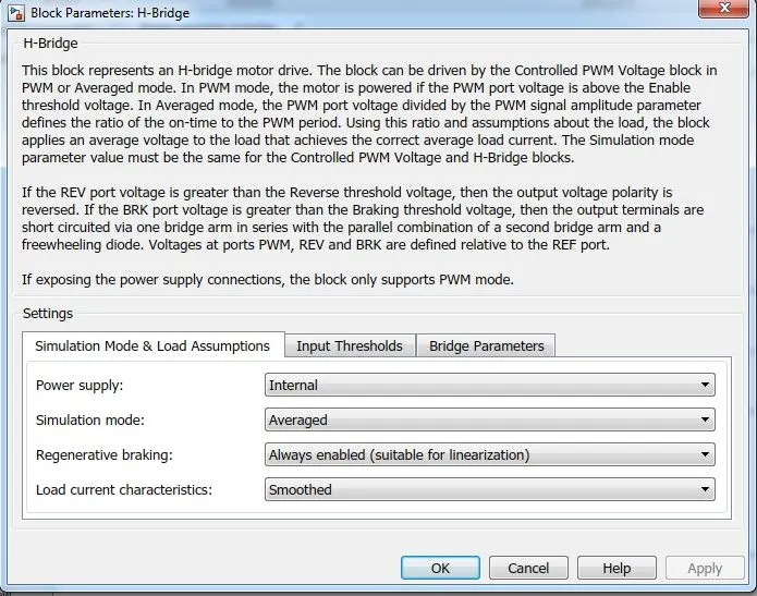
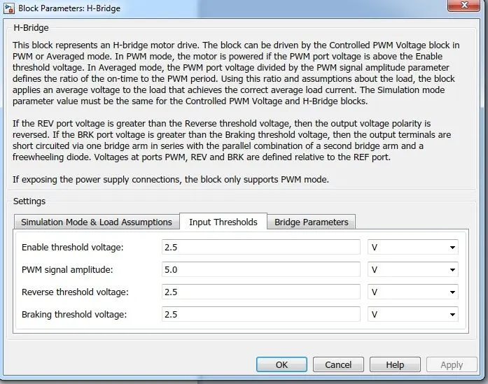
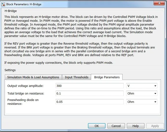
The positive terminal of the H-Bridge is connected with a positive terminal port and the negative terminal of the H-Bridge is connected with a Ground terminal port.
From the power converter block, the positive terminal is connected with the positive terminal of the battery subsystem block and the ground is connected with the ground terminal of the DC motor subsystem block.
Battery System:
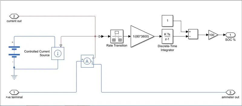
The battery source block is connected with a controlled current source through which rate transition block, gain blocks, and discrete-time integrator blocks are used for getting SOC outport.
1. Battery:
This block models a battery. If you select Infinite for the Battery charge capacity parameter, the block models the battery as a series of internal resistance and a constant voltage source. If you select Finite for the Battery charge capacity parameter, the block models the battery as a series of internal resistance plus a charge-dependent voltage source defined by:
V = Vnom*SOC/(1-beta*(1-SOC))
where SOC is the state of charge and Vnom is the nominal voltage. Coefficient beta is calculated to satisfy a user-defined data point [AH1, V1].
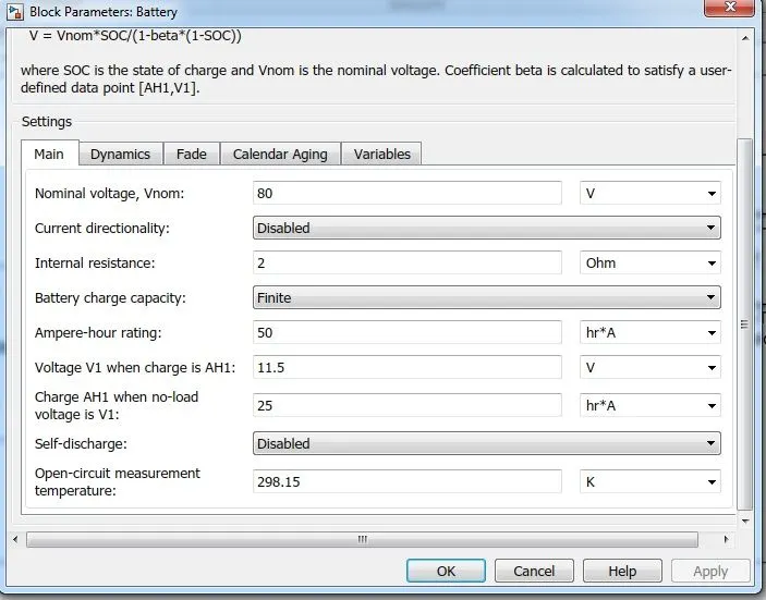
Here I am using 80v, 50Ah battery for the model because the vehicle accelerates, the battery gets discharged and gets charged through the regenerative braking operation. The battery is connected with a controlled current source through which the supply is passed on to the rate transition block.
The rate transition block is used to transfer the data between different rates and tasks. This block is connected with the gain block of (1/(80*3600)) and gain values are applied to the discrete integrator.
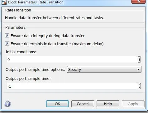
2. Discrete Integrator:
This block is used for discrete time integration or accumulation of the input signal. this block outputs the amount of charge used by the battery.
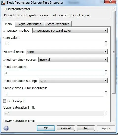
The subtracter block is used here to subtract the value from the gain block with the constant value 1 and the output value of those blocks is multiplied with a gain value of 100. Then the gain block outputs the state of charge in %.
The output port of the current sensor is connected with the positive terminal of the DC motor.
Permanent Magnet DC Motor:
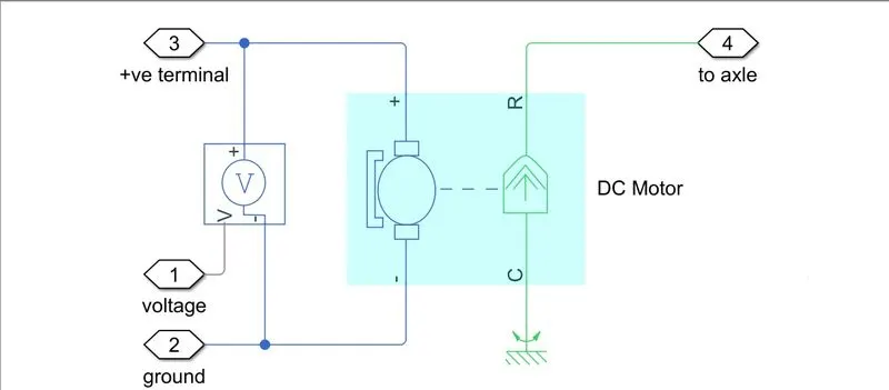
This block represents the electrical and torque characteristics of a DC motor. Here, the current from the battery flows through the positive terminal of the motor to the negative terminal, a torque acts from mechanical C to R ports. The voltage sensor is connected parallel to the DC motor.
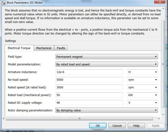
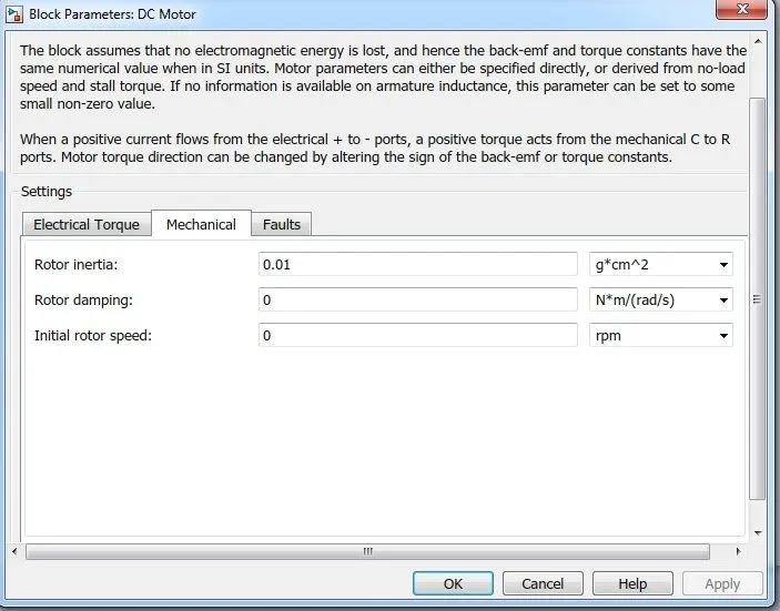
The above picture shows the parameter values we have given for the DC motor,
The motor rated voltage is a 48V DC supply
The motor rated mechanical power is 50KW
No-load speed is 5000 rpm
The rated load speed is 3000 rpm
Rated mechanical load power is 50kW
The C port is connected with a mechanical rotational reference and the R port is connected with the simple gear transmission block of the vehicle body subsystem.
Vehicle Body:
In the vehicle body subsystem, we are taken a vehicle body connected with a simple gearbox and Four tires.
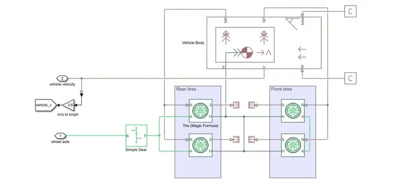
1. Simple Gear:
Represents a fixed-ratio gear or gearbox. No inertia or compliance is modeled in this block. You can optionally include gear meshing and viscous bearing losses.
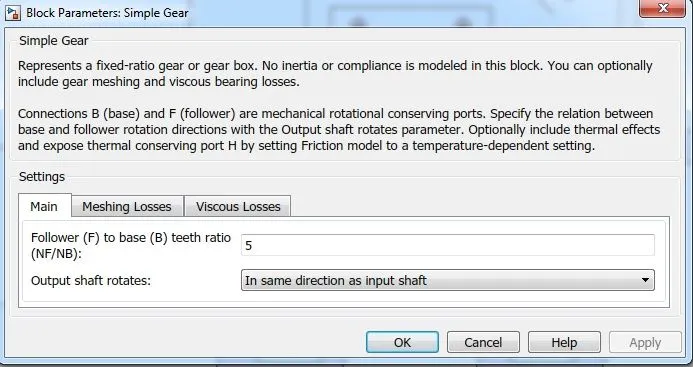
Here the gear ratio is given as 5 and the output shaft rotates in the same direction as the input shaft. Then the gear is connected with the axle-wheel of the tire.
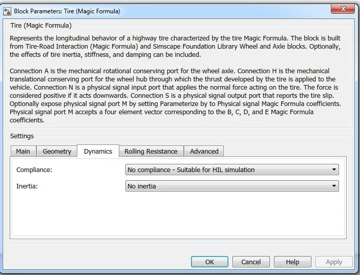
2. Tire:
The tire represents the longitudinal behavior of a highway tire characterized by the tire Magic Formula. The block is built from Tire-Road Interaction (Magic Formula) and Simscape Foundation Library Wheel and Axle blocks. Optionally, the effects of tire inertia, stiffness, and damping can be included.
A is the mechanical rotational conserving port for the wheel axle.
H is the mechanical translational conserving port for the wheel hub through which the thrust developed by the tire is applied to the vehicle.
N is a physical signal input port that applies the normal force acting on the tire.
S is a physical signal output port that reports the tire slip.
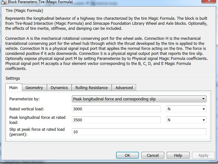
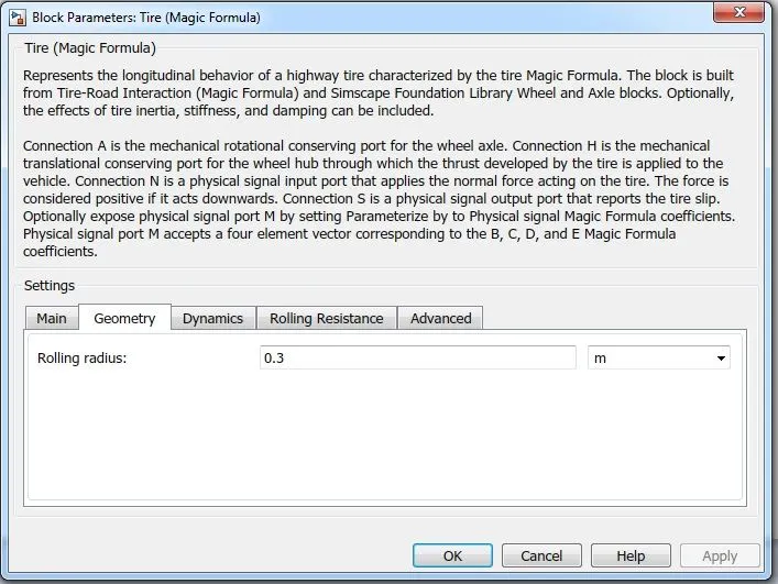
The values given for the parameters are shown below:
3. Vehicle Body:
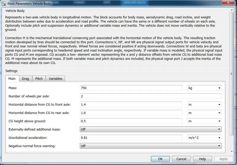
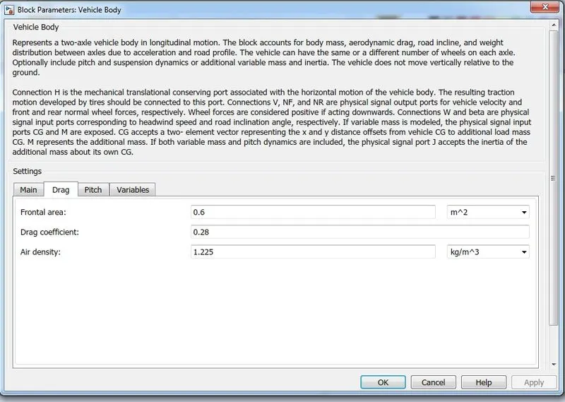
The vehicle body block represents a two-axle vehicle body in longitudinal motion. The block accounts for body mass, aerodynamic drag, road incline, and weight distribution between axles due to acceleration and road profile. The vehicle can have the same or a different number of wheels on each axle.
H is the mechanical translational conserving port associated with the horizontal motion of the vehicle body.
V, NF, and NR are physical signal output ports for vehicle velocity and front and rear normal wheel forces, respectively.
W and beta are physical signal input ports corresponding to headwind speed and road inclination angle, respectively.
The velocity of the vehicle is taken out from the 'V' port and gradeability is given through the 'beta' port and the beta port is connected with PS constant block where we can change the values.
Wind Velocity is given through the 'W' port and it is also connected with the PS constant block. the values assigned for the parameters are shown below:
The Velocity of a vehicle is given as an input for calculating the distance.
Distance Calculation:
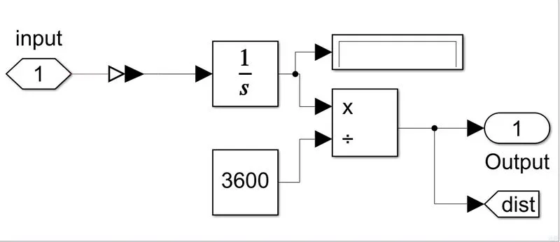
The total distance traveled is calculated by taking velocity as input and the input value is integrated through the integrator block. To get the output in kilometres, we are dividing the value from the integrator block with a constant value of 3600.
Energy Calculation:
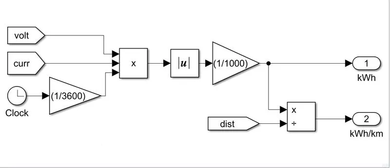
Energy= Voltage*current*time
Energy consumed per kilometer is calculated by dividing the energy by the total distance covered.
Results:
1. Drive Cycle Plot:
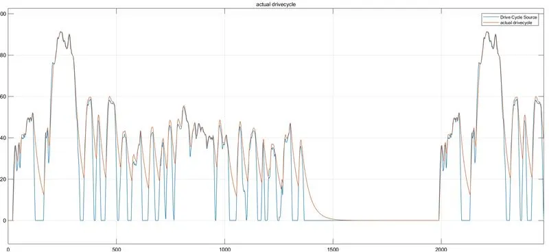
The above graphical representation represents the value of the drive cycle of both the command drive cycle and the actual drive cycle. The increase in velocity represents the acceleration and the decrease in velocity represents the deceleration.
2. Current Plot:
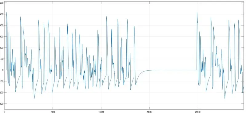
The current is increasing in the case of vehicle acceleration and decreasing in the case of regenerative braking. At last the current goes to the negative state in the case of the battery gets charging.
3. SOC Plot:
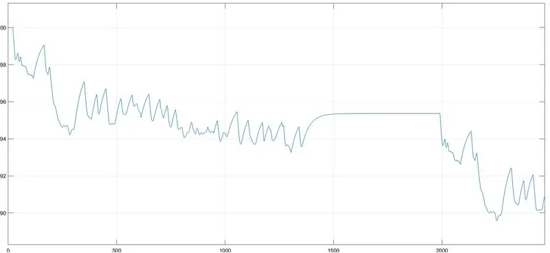
The state of charge is used for measuring the remaining charge left in the battery. At the initial stage, SOC is at 100%, when the vehicle starts accelerating, the current gets dropped and the battery starts discharging. When the vehicle starts decelerating, SOC gets increasing due to regenerative braking and the battery starts charging. SOC remains constant, at the stage of no acceleration or no braking.
4. Voltage Plot:
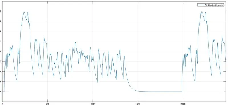
The voltage gets varies according to the drive cycle. The voltage increases when the velocity is high and the voltage gets decreases according to it.
Conclusion:
The Matlab model of an electric vehicle is designed by using a battery and a DC motor. The simulation and results are plotted and verified using the scope block. The output of the voltage, current, and state of charge is executed.