Final Project: Design of an Electric Vehicle

Aim :

• Design of an Electric Vehicle

Objective :

• Create a MATLAB model of an electric car that uses a battery and a DC motor. Choose suitable blocks from the Powertrain block set.

# System-level configurations

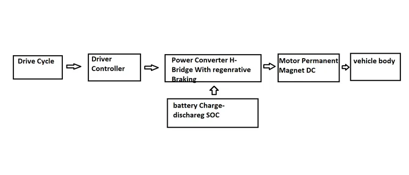
while the design of the electric vehicle we have not considered the actual parts of the vehicle. With the consideration of the system-level configuration, we have created the Matlab model. system-level configuration means we have taken the vehicle body as one system, motor permanent magnet as one system, power converter H-bridge, battery charge or discharge, driver controller and drive cycle as one system.

Matlab model of Electric Vehicle :

link:https://drive.google.com/file/d/1RKyWlhsZjeKFMtzyeNZisrxe6LHoRVIz/view?usp=sharing

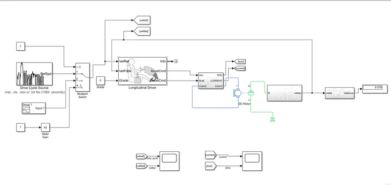
#Explanation of each block used in the EV model :

So, We can start from the last block vehicle body system

block vehicle body system :

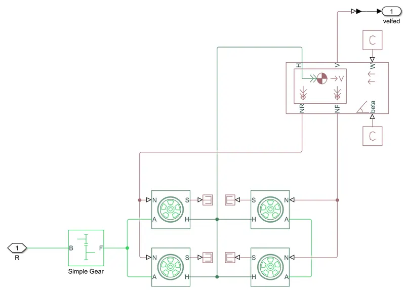
In the Vehicle, the body system contains Tire Block, Vehicle Body Block, and simple gear block. Here In the above, we used the four-tire block which acts as an actual car four-tire. All tire hub point is connected to the Hub point of the vehicle body block. Two rear tire N point is connected to the rear of NR point of the Vehicle body. Two front tire N points Connected to the NF point of the Vehicle body. The connection which is not required is terminated using the PS Terminator Block.PS constant block is used to connect the wind and beta connection containing the zero value. The rear two tires are connected using the axis connection and the front two tires also. At the rear axial we connected the simple gear.

Vehicle body block :

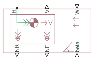
The Vehicle Body block represents a two-axle vehicle body in longitudinal motion.

The Vehicle Body block lets you model only longitudinal dynamics, parallel to the ground and oriented along the direction of motion. The vehicle is assumed to be in pitch and normal equilibrium. The block does not model pitch or vertical movement. As such, the equations assume that the wheels never lose contact. This constraint can result in negative normal forces.

The vehicle body has the following type of ports:

NR - Rear axial normal force, is positive when acting in the downward direction.

NF - Front axial normal force, is positive when acting in the downward direction.

beta - Road Incline angle, rad

W - Headwind speed, m/s

V - Longitudinal velocity, m/s

H - Horizontal motion

Conserving port associated with the horizontal motion of the vehicle body. Connect tire traction motion to this port.

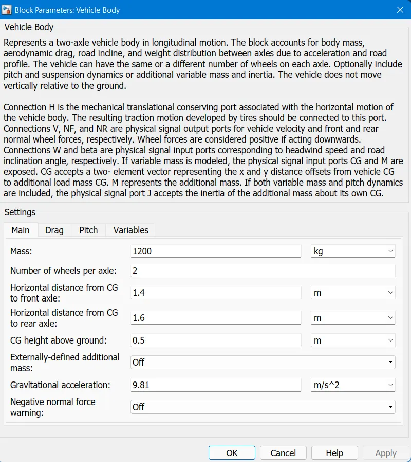
In the Vehicle body, we can add the actual data of the vehicle eg. Mass, number of wheels on the axle, CG, and many things about the Vehicle.

Tire (Magic Formula) block :

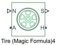
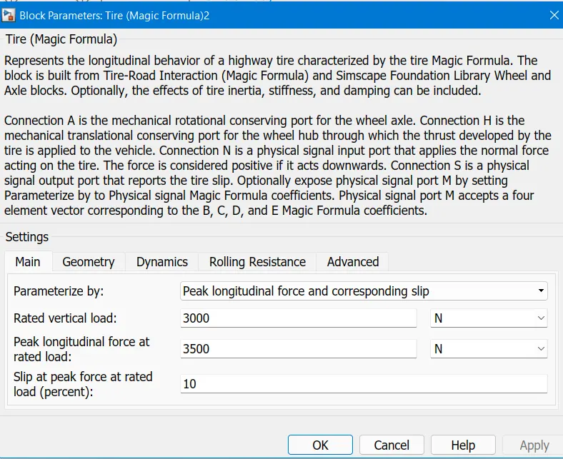
Represents the longitudinal behavior of a highway tire characterized by the tire Magic Formula. The block is built from Tire-Road Interaction (Magic Formula) and Simscape Foundation Library Wheel and Axle blocks. Optionally, the effects of tire inertia, stiffness, and damping can be included.

The Tire (Magic Formula) block models the tire as a rigid wheel-tire combination in contact with the road and subject to slip. When torque is applied to the wheel axle, the tire pushes on the ground (while subject to contact friction) and transfers the resulting reaction as a force back on the wheel. This action pushes the wheel forward or backward. If you include the optional tire compliance, the tire also flexibly deforms under load.

Tire Block Contains the following ports :

N - Normal Force, The normal force is positive if it acts downward on the tire, pressing it against the pavement.

S - Slip, relative slip between the tire and road.

A - axle that the tire sits on.

H - port associated with the wheel hub that transmits the thrust generated by the tire to the remainder of the vehicle.

Simple Gear block :

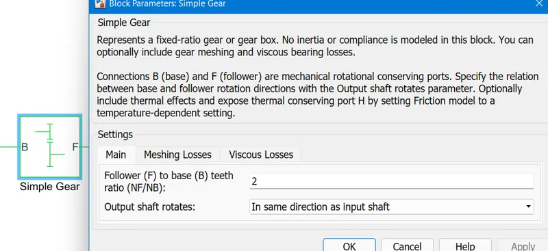
Here in the simple gearbox B and F are the mechanical rotational conserving ports.

DC Motor Block :

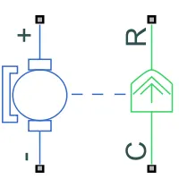
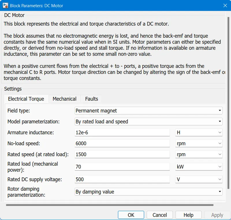
This block represents the electrical and torque characteristics of a DC motor.

The block assumes that no electromagnetic energy is lost, and hence the back-emf and torque constants have the same numerical value when in SI units. Motor parameters can either be specified directly or derived from the no-load speed and stall torque. If no information is available on armature inductance, this parameter can be set to some small non-zero value.

When a positive current flows from the electrical + to - ports, a positive torque acts from the mechanical C to R ports. Motor torque direction can be changed by altering the sign of the back-emf or torque constants.

Power Elctronic System :

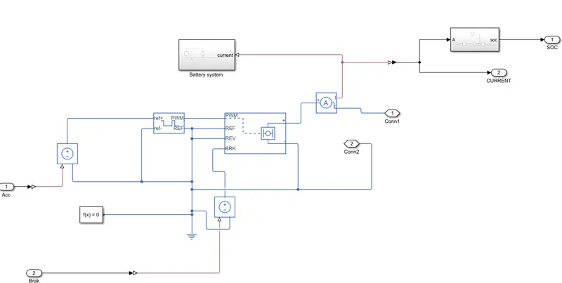
In the above system H-bridge block, the Controlled PWM voltage block, the controlled voltage block, and the current sensor are used.

H-bridge Block :

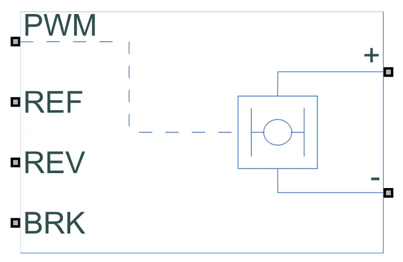
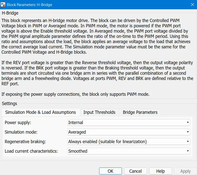
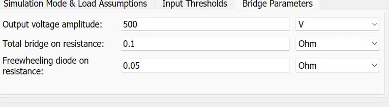
The H-Bridge block represents an H-bridge motor driver. The block has the following two Simulation mode options:

PWM and Averaged simulation mode.

And Averaged mode has two current characteristics

• smooth
• unsmooth or discontinuous

Controlled PWM voltage Block :

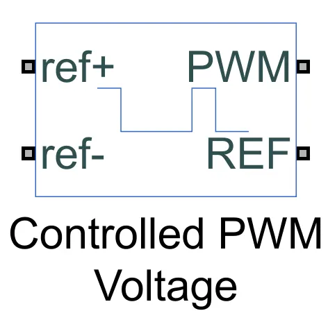
controlled PWM voltage consists of the four ports

ref+ electrical reference voltage.

ref - Negative electrical reference voltage

PWM Electrical conserving port associated with the pulse-width modulated signal

REF port associated with the floating zero volt reference.

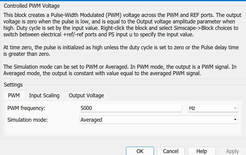
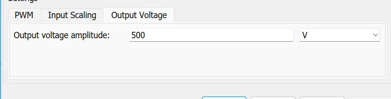
In the H bridge block, we used the Averaged simulation mode and load current characters as smooth. So this Hbrodge block required the PWM voltages created by Controlled PWM voltages. Where ref+ input is given through the controlled voltage source. input to that controlled voltage source is the longitudinal drivers gives acceleration as output. As per the acceleration output, the voltage is pass to the controlled PWM voltage block. As the same way braking ports are connected

One thing that increases the simulation time if we use the different simulation methods in Controlled PWM and H-bridge block

Battery system :

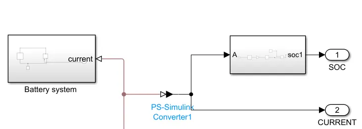
In the battery system, we use the simple battery that the battery draws the current as per current senses for the load.

where we used the current sensor.

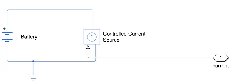
battery :

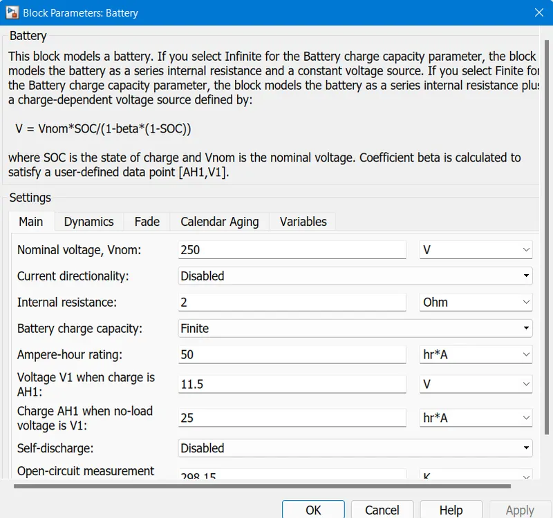
we put the battery voltage as we required for the motor 250

controlled current source :

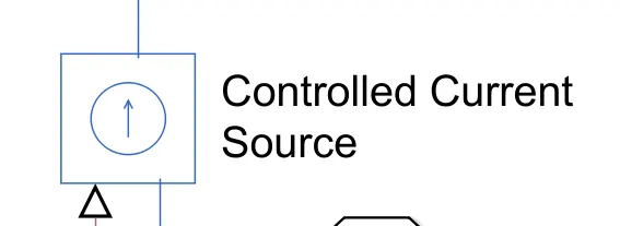
controlled current source block supply the current as per some input. the current value we get at the load with the current sensor we applied the input for the controlled current source.

SOC calculation :

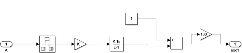
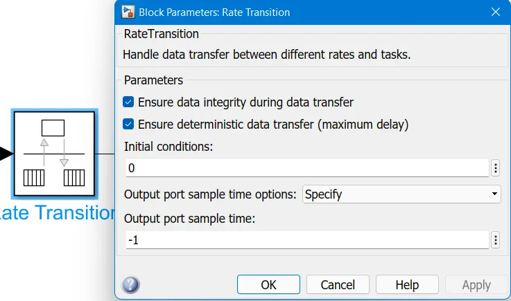
it handles the current we get at a different rate.

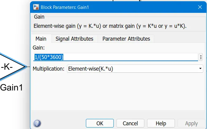
After that, it connected to the gain block. the gain will multiply the value of k = 1/A*sec, Where in this battery capacity is A.hr so, in our case the value is 50. k = 1/(50*3600)

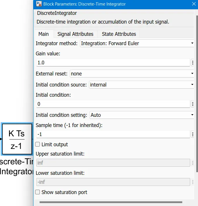
then that gain value is pass to the discrete-time integrator block and the output we get is subtracted from the one where one is considered as the 100% charged. again multiplied by 100 which gives in percentage soc.

Longitudinal Driver Block :

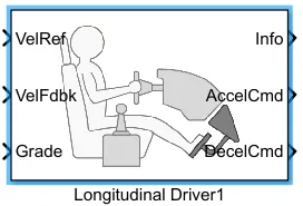
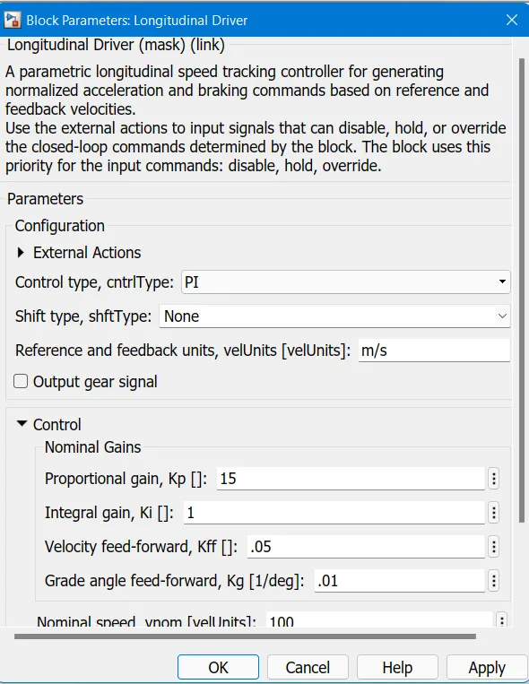
The Longitudinal Driver block implements a longitudinal speed-tracking controller. Based on reference and feedback velocities, the block generates normalized acceleration and braking commands that can vary from 0 through 1. You can use the block to model the dynamic response of a driver or to generate the commands necessary to track a longitudinal drive cycle.

Drive cycle :

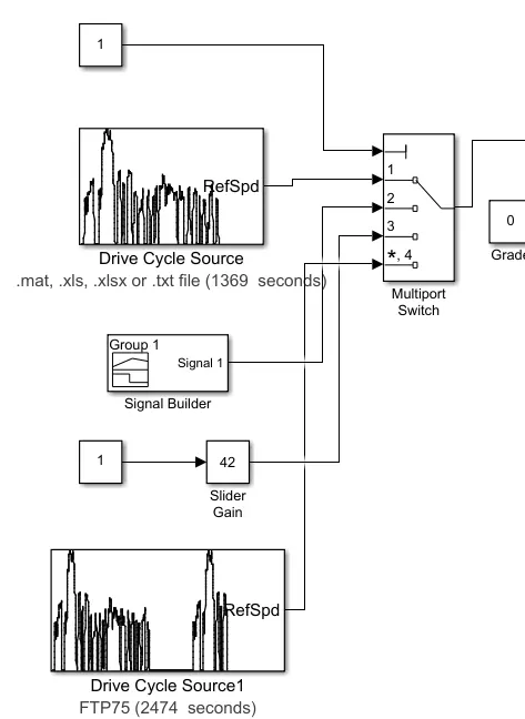
Here I have used the two types of drive to compare the same motor for different drive cycles.

also, I have introduced some different methods that can generate the drive cycle data.

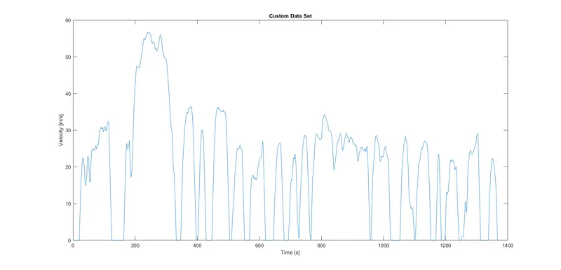
UDDS drive cycle :

Urban Dynamometer Driving Schedule (UDDS) driving cycle is a typical urban driving cycle with an average speed of 31.51km/h and has frequent braking and acceleration.

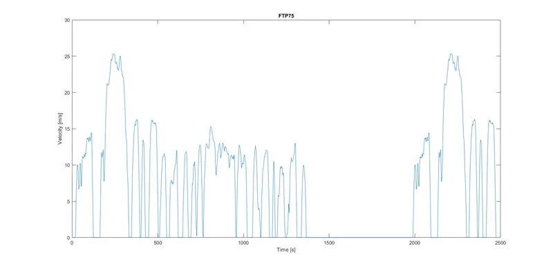
FTP75 drive cycle :

FTP75 is a mandatory dynamometer test on tailpipe emissions of a car that represents the driving conditions of the city, which was developed from the Urban Dynamometer Driving Schedule (UDDS, also known as FTP-72). As shown in Figure 7, FTP75 is identical to UDDS plus the first 505 s of an additional UDDS cycle

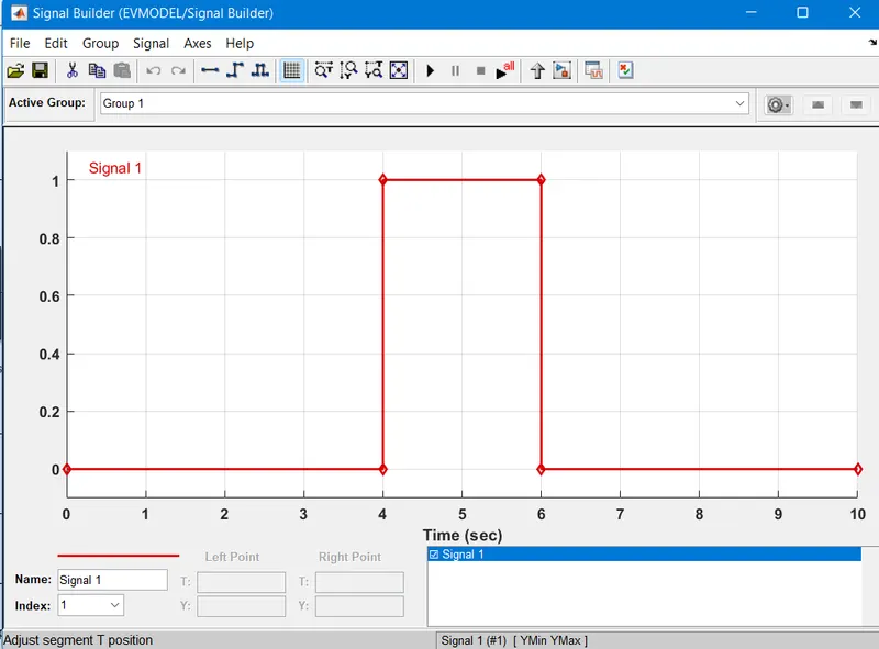
Signal builder :

slider gain :

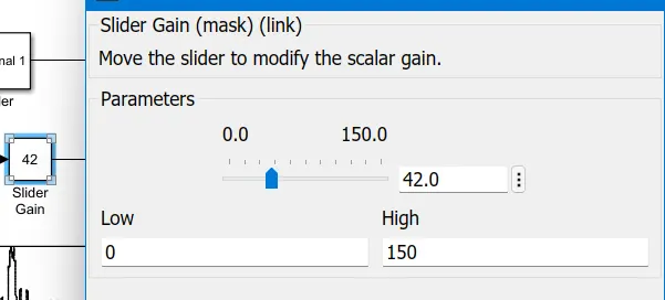
The Slider Gain block performs a scalar gain that you can modify during simulation. Modify the gain using the slider parameter.

Multiport switch :

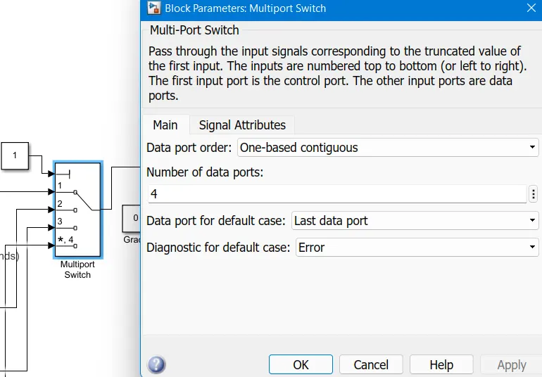
Multiport acts as a switch in that first are port is the controller port and other is the data port. With controlled port which can control which data port should be accepted

Distance calculation :

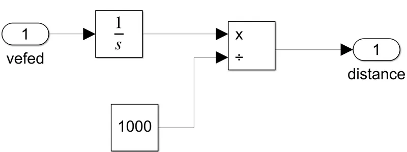
In that, we integrate the speed which gives distance and then divided by 1000 which convert them to Km.

#Results :

DC permanent magnet motor with 250 volt DC rated supply voltage having the rated load around 70 kW, no-load speed 6000 and rated speed or at load is 1500 rpm

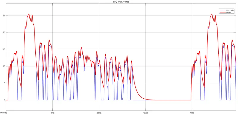
From that, we can say this type of motor can easily overcome the FTP75 drive cycle. This drive cycle runs around 2474 sec.

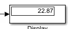
with the above drive cycle, it covers a distance is 22.87 km.

Current and soc % results :

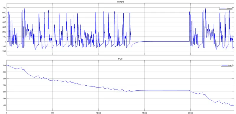
From the above results, we get that with the above type of dc motor and run vehicle with FTP75 drive cycle battery not drain totally it still have the 40 % battery remains.

For the same DC motor that I have mentioned above, I run the UDDS drive cycle.

Results we get for the UDDS drive cycle :

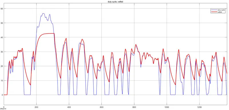
From the above results, we can say that feedback velocity somewhat matches with the drive cycle velocity. with the same DC motor parameter vehicle not being able to go the drive cycle max speed

Results of SOC % and currents :

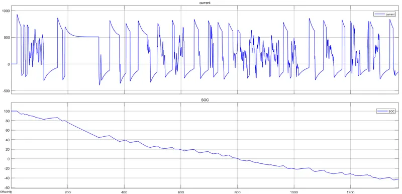
From the above results, we get that the motor is drained around 800 sec.

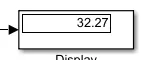
The vehicle can able to travel 32.27 km

#Conclusion :

• we understood the block of the powertrain
• we created the full Electric vehicle model using the Matlab