FINAL INDEPENDENT PROJECT

Aim-

Program in MATLAB for simulation of air standard DIESEL cycle.

Objectives:-

1. To study working on diesel
2. To calculate thermal efficiency of cycle using state variables
3. To plot graph pv diagram using state variables

Introduction:-

It is a combustion process of reciprocating IC engine. In it fuel is ignified by heat generated during the compression of air in the combustion chamber into whhich fuel is then injected.this is in contrast to igniting the air-fuel mixture with a spark plug as in the otto cycle. Diesel engine are used in aircraft, automobiles, power generation, diesel electric locomotive, and both surfacr ships and submarines.

Theory:-

This process is ideal, combustion is replaced by heat addition to the air, and exhaust is replaced by a heat rejection process which restores the air to the initial state.

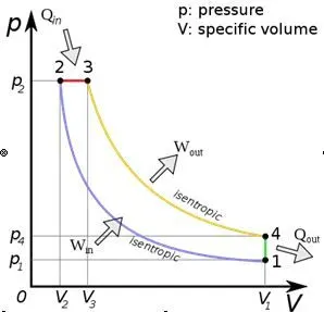
Process 1-2 is the adiabatic compression process. In this process temperature of the air increases during the compression process and with a large compression ratio it will reach the ignition temperature of the injected fuel.

Process 2-3 is the contant pressure process. its also known as isobaric process. In this process the burnt gasses are simply exhausted and replaced by a fresh charge of air.

Process 3-4 is the adiabatic expansion process. In this process ithe inside air is expand and then the power will be generated mixture of air-fuel piston goes down.

Process 4-1 is the constant volume process. In this process heat is removed from the system by flushing out the combusted gases.

Inputs:-

Bore of engine (D) = 0.20 (m) Stroke length (L) = 0.30 (m) Connecting rod (Conrod) = 0.42 (m) Cut off = 8% = 8/100 = 0.08 Compression ratio (Cr) = 15

p1 = 1 (bar) = 1*10^5 (Pa)

t1 = 27 (C) = 27+273 = 300 (k)

gamma = 1.4

Process:-

1. Start the program clearing all back
2. Put all inputs and calculate swept volume, clearance volume, cut off
3. Calculate all state variables point like pressure at point 2,3,4 and temp at point 2,3,4 using ideal gas
4. Create function calculating of actual total volume of piston we call the func name as actual_volume which have one output variable and six geometric parameters which are
5. After calculation of actual total volume we can calculate compression and expansion volume for plotting the pv
6. For the calculation of compression volume crank angle will be change in 180 to 0 same as expansion volume 0 to 180.
7. After calculation all equation we can give plot
8. Labeling x and y axis and give title name for graph

Main code:-

clear all 
close all 
clc

%inputs
D = 0.20;	%cylinder diameter or  bore  of  cylinder  in [m] 
L = 0.30;	%stroke length in [m]	
conn_rod = 0.42;	%Connecting rod length in [m]
Cr = 15;	%Compression ratio 
cutoff = 8/100;
%Calculate cut off ratio
%COr = cut off ratio
%cut_off = (COr-1)/(Cr-1)
%COr-1 = (Cr-1)*Cutoff 
COr = (Cr-1)*cutoff+1;
gamma = 1.4;	%cp/cv constant

%State variables
p1 =  1*10^5; %pressure at point 1 in [pascal] 
t1 = 27+273;	%temp at point 1 in [kelvin]

%Calculate Swept Volume & Clearance  Volume 
Vs  =  pi/4*D^2*L;	%swept volume
Vc  =  Vs/(Cr-1);	%clearance volume

%Isentropic compression process
%State variables at point  1-2  
v1 = Vs+Vc;

constant = p1*v1^gamma;
V_comp = prac(D,L,Cr,conn_rod,180,0); 
P_comp = constant./V_comp.^gamma;

%Constant pressure heat addition process
%state variables at point 2-3 
v2 = Vc;
%p2*v2^gamma = p1*v1^gamma
%Cr = v1/v2
p2 = p1*(Cr)^gamma;
%t2/t1 = (v2/v2)^(gamma-1) 
t2 = t1*(v2/v1)^(gamma-1);

%state variables at point 3-4
%COr = v3/v2 
v3 = COr*v2;
p3 = p2;	%pressure at point 2 & 3 are remains same
%t3/t2 = v3/v2 
t3 = t2*(COr);

constant = p3*v3^gamma;
V_exp = prac(D,L,Cr,conn_rod,0,180); 
for i = 1:length(V_exp);
    if V_exp(i)<v3; V_exp(i)=v3;
    end
end
P_exp = constant./V_exp.^gamma;

%state variables at point 4-1
v4  =  v1;	%volume at point 1 & 4 are remains same
%p3*v3^gamma = p4*v4^gamma 
p4 = p3*(v3/v4)^gamma;
%t4/t3 = (v4/v3)^(gamma-1)
t4 = t3*(v4/v3)^(gamma-1);

%efficiency of diesel cycle	[Nth]
%Nth = 1-(1/gamma*(Cr)^(gamma-1))*[COr^gamma-1/COr-1] 
term1 = 1/(gamma*(Cr)^(gamma-1));
term2  =  (COr^gamma-1)/(COr-1); N = 1-term1*term2
Nth = N*100

%plotting 
hold on
plot(v1,p1,'*','color','k')
plot(V_comp,P_comp,'color','k')
text(v1,p1,'State 1','color','g')
plot(v2,p2,'*','color','k')
text(v2,p2,'State 2','color','g')
plot(v3,p3,'*','color','k')
plot(V_exp,P_exp,'color','k')
text(v3,p3,'State 3','color','g')
plot(v4,p4,'*','color','k')
text(v4,p4,'State 4','color','g')
line([v2  v3],[p2 p3],'color','k')
line([v4 v1],[p4 p1],'color','k') 
title('PV Diagram "Diesel Cycle"') 
xlabel('Volume')
ylabel('pressure')

Function Code:

clear all
close all
clc
function V = prac(D,L,Cr,conn_rod,start_crank,end_crank)
%D = 0.20;	%bore
%L =  0.30;	%stroke
%Cr = 15;	%compression ratio
%conn_rod = 0.42;	%connecting rod

a = L/2;
R = conn_rod/a;

theta = linspace(start_crank,end_crank,100);

%calculate swept volume and clearance  volume 
Vs = (pi/4)*D^2*L;
Vc = Vs/(Cr-1);

%calclute formula
%V/Vc = 1+0.5*(Cr-1)[(R+1-cosd(theta)) - (R^2-sin(theta)^2)^0.5] 
term1 = 0.5*(Cr-1);
term2 = R+1 - cosd(theta);
term3 = (R^2 - sind(theta).^2).^0.5;

V  =   (1+term1*(term2-term3)).*Vc; 
end