FINAL INDEPENDENT PROJECT
wood chip fired and municipal waste fired combined heat and power plants
Terms
B1 Brista 1 Combined Heat and Power Plant
B2 Brista 2 Combined Heat and Power Plant
BP Backpressure mode
CFB Circulating Fluidized Bed
CHP Combined Heat and Power
DC Direct Condensing mode
DHW District Heating Water
FGC Flue Gas Condensation
HHV Higher Heating Value (of a given fuel)
O&M Operations & Maintenance
List of variables
This is a list of variables which will be used in the equations in the following chapters.
m Total steam mass flow rate
mx Steam mass flow rate in steam extraction x
mdhw Mass flow rate of district heating water
mair Mass flow rate of combustion air for preheating (Brista 2)
hx Enthalpy of stream x
hin Enthalpy of district heating water entering first condenser
hint Enthalpy of district heating water leaving first condenser
hout Enthalpy of district heating water leaving second condenser
dtx Temperature difference of stream x
cpx Specific heat of stream x
px Pressure at point x
Tx Temperature at point x
ηx Efficiency of component x
Qx Thermal power input/output to/from component x
Px Electrical power input/output to/from component x
Mx Molar mass of chemical species x
Cx Concentration of chemical species x
px Average spot price of x during a given hour
cx Total operating cost of x during a given hour
Introduction
The Brista 1 plant is a wood chip-fired combined heat and power (CHP) plant with a maximum thermal
power output of 130 MW and a maximum electrical power output of 42 MW located near Märsta,
northwest of Stockholm, Sweden. The primary purpose of the plant is to supply heat to the northwest
district heating grid.
In order to meet increasing demand for district heating, Fortum Heat is constructing a second CHP plant
next to Brista 1. The Brista 2 plant will have a thermal power output of 60 MW and an electrical power
output of 20 MW using a mixture of municipal and industrial waste as fuel.
Due to changes in the European Green Certificate program, the fuel subsidies for wood chips will be
significantly reduced. This will cause the Brista 1 plant to incur significantly increased operating costs. The
Brista 2 plant, however, will not be affected by these changes and will therefore be much cheaper to run
than Brista 1. However, due to the large demand for district heating it will be necessary to run both plants
in parallel at certain times in order to meet the heating demand and/or maximize revenue during periods
of high electricity demand.
In order to run the plants in parallel as profitably as possible, Fortum Heat have expressed interest in
modeling the two power plants and conducting computer simulations in order to formulate an operational
strategy, taking part-load operation and the costs related to starting and stopping the plants into
consideration.
Method
A computer model has been programmed based on the operating characteristics of the two CHP plants.
The computer model takes production costs and potential revenues from electricity production into
account and optimizes the parallel operation of the two plants based on multiple constraints for different
likely operating scenarios.
Objectives
This project has studied the parallel operation of the Brista 1 and Brista 2 CHP plants from a production
cost perspective. This involved thermodynamic and economic modeling of the two plants and
programming an optimization program to determine the best possible operating strategy for their parallel
operation.
Constraints
The modelling has been limited to the Brista 1 and Brista 2 plants. The rest of the northwestern district
heating grid is not a part of the model.
The Plants
Brista
Overview
The Brista 1 plant features a CFB boiler fueled by wood chips with a rated power output of 122 MW. This
produces steam at a temperature of 540°C and a pressure of 140 bar with a maximum steam flow rate of
50 kg/s. The steam is fed through high- and low pressure turbine stages which both have multiple steam
extractions. The high-pressure steam extractions are used for feedwater preheating, process steam and
boiler inlet preheating. The low-pressure steam extractions are used for preheating condensate and to
provide steam for two separate condensers which operate at different pressures.
The plant has also been retrofitted with a flue gas condensation unit, which provides an additional 30 MW
of thermal power output at maximum steam load.
2 Plant layout
Backpressure mode
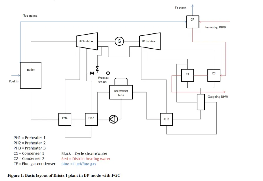
Operating modes
The plant can be run in three different modes – backpressure mode, direct condensing mode and mixed
mode. In backpressure mode, the steam from the boiler is fed through both turbines and then passes
through condenser 1 and 2. The condensers operate at two different pressure levels, and for this reason
the steam reaching condenser 2 is extracted from the low-pressure turbine prior to full expansion. In this
mode, the plant produces both electricity and district heating.
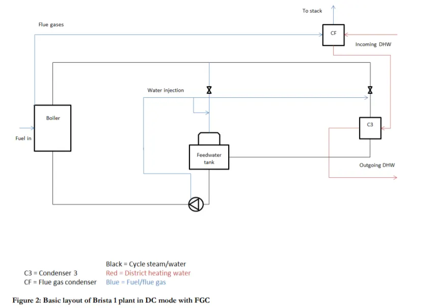
In direct condensing mode, the steam from the boiler completely bypasses the turbines and is fed into
condenser 3. Before it can be fed into the condenser, however, the steam is expanded to a lower pressure
and water is injected in order to lower the temperature to an acceptable level for condenser operation.
This water is extracted between two stages in the feedwater pump at a pressure of around 40 bar. The
increased mass flow of lower-pressure steam creates a larger mass flow of steam through the condenser
than in backpressure mode. In this mode, the plant produces no electricity but produces significant
amounts of district heating.
In mixed mode, part of the steam is fed through the turbines and part is fed directly to condenser 3. This
can be viewed as a hybrid of the two previously described operating modes. In this mode, the plant
produces both electricity and district heating; however the electricity production is lower than it would be
in backpressure mode.
Additionally, all of the above modes can be run with or without the flue gas condensation module. In the
Brista 1 plant, the flue gas condensation and flue gas cleaning systems are separate.
4 Operating Range
The maximum plant thermal power output is 113 MW and the minimum stable thermal power output is
43 MW. In addition, condenser 3 is limited to a thermal power output of 85 MW and the two turbines
have a combined maximum electrical power output of 42 MW and a minimum stable electrical power
output of 12.6 MW. The flue gas condensation system has a maximum thermal power output of 30 MW
and a minimum of 15 MW
Process modeling
In order to keep the size of the project manageable, it was decided that the only operating modes that
should be considered are:
1) Brista 1, Backpressure mode
2) Brista 1, Direct Condensing mode
3) Brista 2, Backpressure mode
The reason for this was that mixed mode was found to be very hard to model and that running Brista 2 in
direct condensing mode was determined to be an unlikely scenario.
Mathematical modeling
Boiler thermal power output and fuel input
Since the total district heating load is an input parameter, the required heat output of each plant is known
beforehand. Using a known boiler efficiency and heating value for the fuel, it is therefore possible to
compute the necessary boiler thermal power output for a given steam flow independently of the
mass/energy balances for the steam system. This, in turn, allows the fuel flow to be computed using the
higher heating value (HHV).
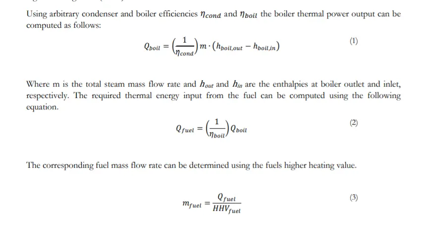
Using arbitrary condenser and boiler efficiencies and the boiler thermal power output can be
computed as follows:
Energy and mass balances
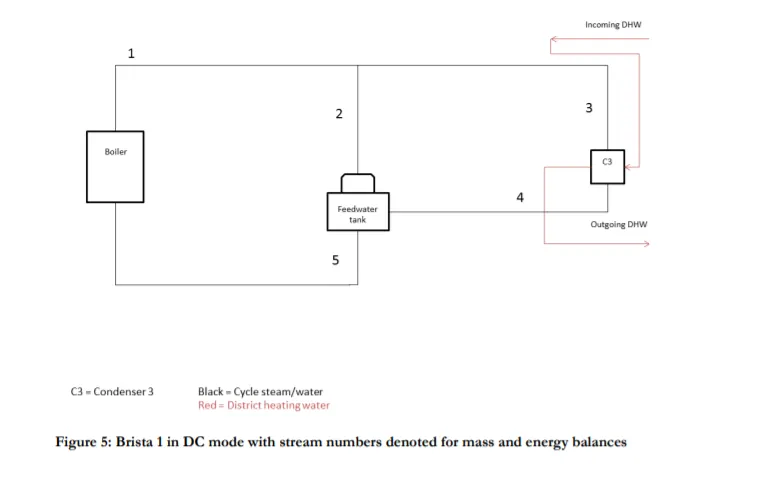
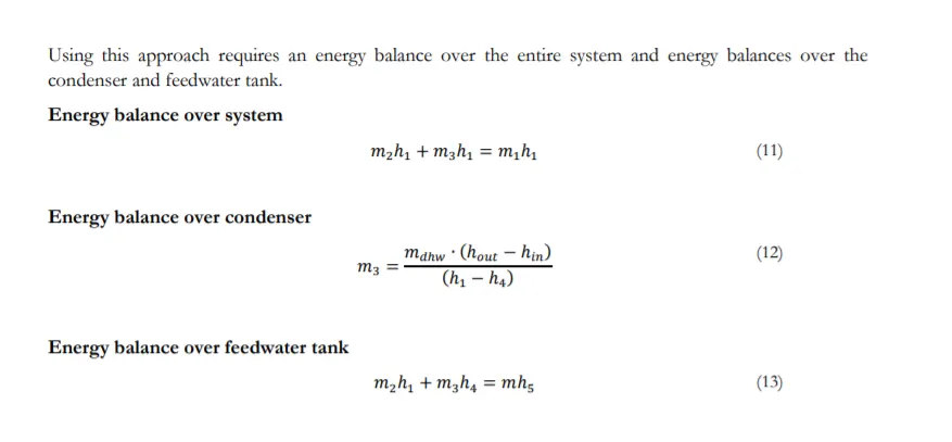
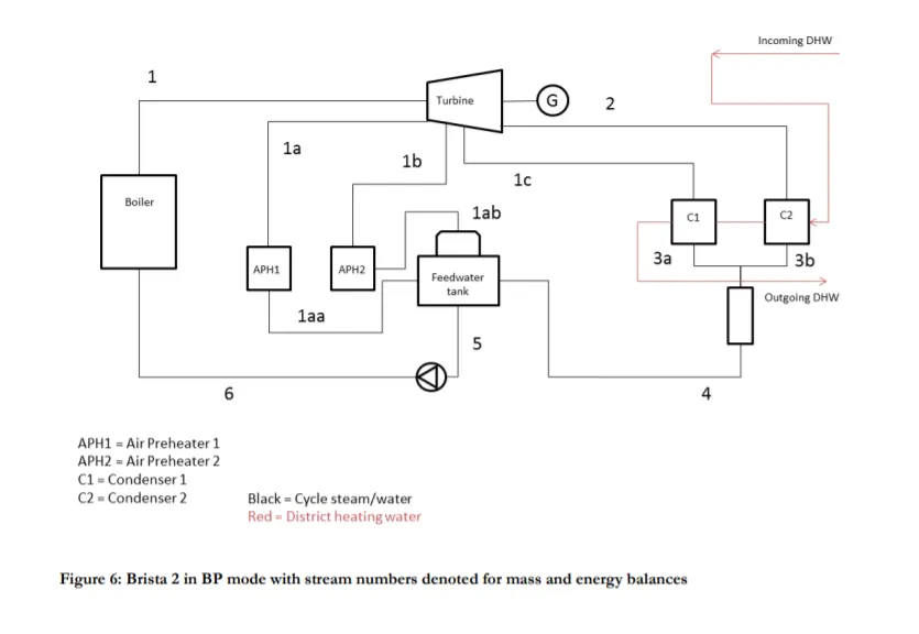
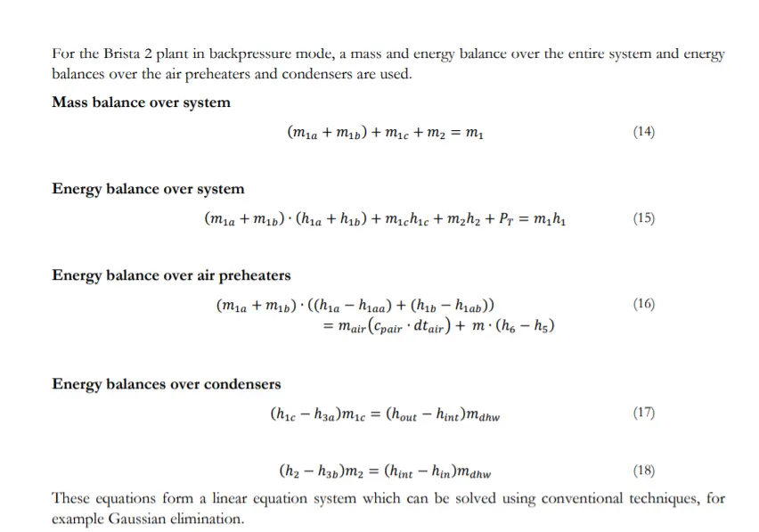
Based on the flow sheets illustrated in Figure 1, Figure 2 and Figure 3, sets of mass and energy balances
were constructed for each operating mode. The purpose of these balances is to compute the steam flow in
each branch of the system, i.e. the size of the steam extractions. This is necessary in order to determine
the turbine power output and the thermal power output from the condensers. The thermal power
contribution from the flue gas condensation system is treated independently of these mass/energy
balances. This is explained further in section 6.1.2.4.
The number of energy and mass balance equations for each operating mode is kept at a minimum in order
to ensure that the equation systems they produce are as small as possible. The reason for this is that the computer program which solves the equation systems does so iteratively, so larger systems will result in
significantly longer computation times.
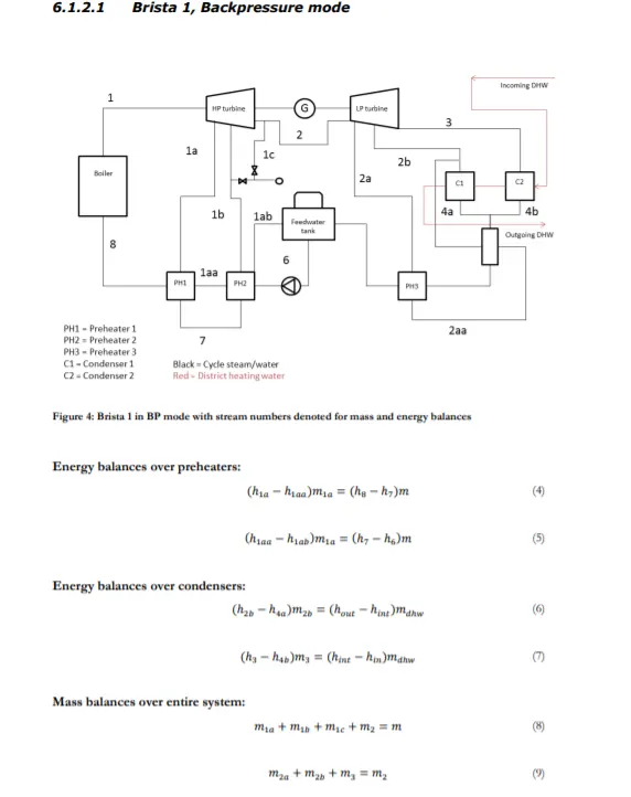
When Brista 1 is run in backpressure mode at low boiler loads, a situation can occur where one of the
steam extractions must be shut off. In this case, an energy balance over the feedwater tank is also used:
Energy balance over feedwater tank:

Brista 1, Direct Condensing mode
In direct condensing mode, the mass and energy balances are significantly simpler than in backpressure
mode. This is because there is only one condenser in direct condensing mode and because there is no
turbine work there are no steam extractions at varying pressures. The complicating factor when modeling
the direct condensing mode is the water injection before the condenser and the feedwater tank. In order
to solve this problem, we disregard the water injection during the calculations.
The purpose of the water injection is to reduce the pressure of the water from the boiler to a level which
the condenser can handle. Effectively, we obtain a significantly larger mass flow rate of steam at a much
lower pressure. This is due to practical considerations such as material fatigue in the condenser. However,
from an energy standpoint, a smaller mass flow rate of higher pressure steam contains the same amount of
energy as a larger mass flow rate of lower pressure steam. Reducing the pressure simply spreads the same
amount of energy throughout a larger volume of water.
Therefore, in order to simplify the simulation, we can disregard the water injection and simply view the
amount of energy in the high pressure steam as equal in magnitude. This allows us to remove the entire
water injection loop from the equation. The model will not be able to solve the actual mass flow rate
through the condenser, but it will be able to solve the heat flow rate through the condenser accurately.
Brista 2, Backpressure mode
In the Brista 2 plant, steam extractions are used to preheat the combustion air entering the boiler before
preheating the boiler feedwater. The thermal energy lost through this process must be incorporated into
the energy balances. The inlet and outlet temperature of the combustion air is known, and the mass flow
rate of air can be approximated using least-squares interpolation from known data points, creating a
function which is dependent on the steam mass flow rate. The specific heat of the air is assumed to be the
average value between the inlet and outlet air temperatures
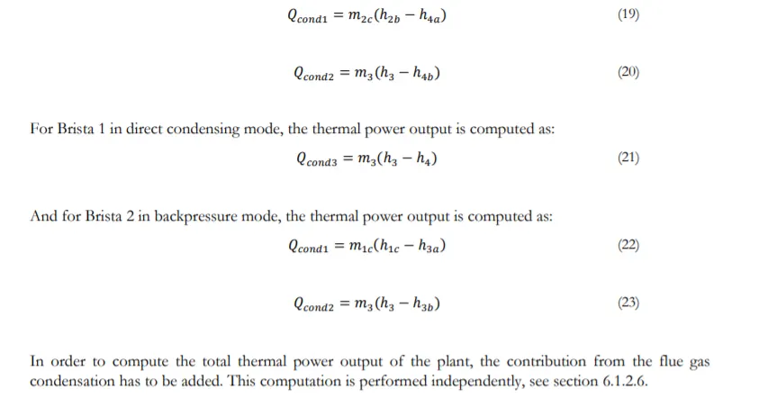
Condenser thermal power output
The thermal power output is computed using an energy balance over the condenser(s) after the mass and
energy balances have been solved for. The reason for this is that all of the steam extractions have to be
taken into account in order for the steam mass flow rate over the condenser(s) to be known.
For Brista 1 operating in backpressure mode, the thermal power output is computed as:
Turbine electrical power output
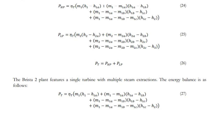
The turbine electrical power output is computed using an energy balance over the turbine(s). Since the
turbine(s) feature multiple steam extractions, these must be taken into account as they effectively reduce
the mass flow through certain sections of the turbine and contribute to a reduced power output.
Since Brista 1 features two turbines – one high pressure and one low pressure – it requires two separate
energy balances.
Combustion and flue gas condensation
The flue gas condensation was treated as an entirely separate system. Since the boiler steam load is used as
a control variable, it is known before the steam system balances have been solved. This means that the
boiler power output can also be computed independently of the steam system mass/energy balances.
Since the boiler power output can be computed, the fuel flow rate and corresponding flue gas flow can
also be computed.
Once the flue gas flow rate has been computed, the amount of heat available in it can also be computed,
and the corresponding flow rate of district heating water which can be heated to the desired temperature
can be computed. This value can then be deducted from the total required flow rate of district heating
water, and the remainder used in the steam system mass/energy balances. This approach avoids
nonlinearities which would otherwise be present and allows the economic benefits of the flue gas
condensation system to be taken into account.
The total district heating water flow rate is effectively split into two parts – one which is covered by the
thermal energy in the flue gases and one which is covered by the combined thermal power output of the
condensers.
Given a dry, ash-free chemical composition and the moisture content of the fuel in question, the flue gas
flow rate can be computed using the following method.
The dry weight percentage of a chemical species X is first converted to a wet-weight percentage by
multiplying it by the moisture content
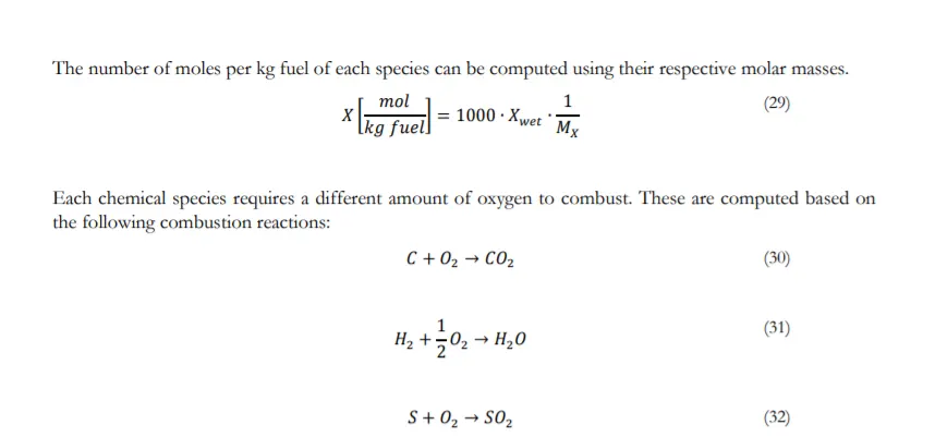
Nitrogen present in the fuel is considered inert and oxygen present in the fuel gives a corresponding
negative contribution to the total oxygen demand. The total oxygen demand is computed as the sum of
each chemical species individual demand. The amount of flue gases produced is computed based on the
same reactions, with the fuel moisture content added to the total water and the nitrogen present in the
combustion air added to the total nitrogen.
The final step is to use the excess air factor and add the corresponding amount of oxygen and nitrogen to
the flue gas composition. Thus, the total gas amount is:

his is the total amount of moles of flue gas produced per kg fuel. In order to compute the mass flow rate
of the fuel, this must be converted from normal cubic meters (Nm3
) into kilograms.

This value represents the amount of flue gases produced per kilogram of fuel burned. It is therefore
multiplied by the fuel flow to give the total flow rate of flue gases at a given operating point
Approximating temperatures and pressures
Both of the plants and their operating modes were modeled using an approach based on energy- and mass
balances combined with extrapolation of known operational data. Energy and mass balances were
constructed for each operating mode and turned into a linear equation system. However, certain
parameters within the model are dependent on external influences such as the temperature difference of
the district heating water and the boiler steam load. These parameters affect the pressures and
temperatures of the streams within the plant.
In order to account for this, several data points were obtained from the operational data of the Brista 1
plant, several years of which was made available by Fortum. For the Brista 2 plant, design estimates were
obtained from the contractors and manufacturers responsible for the construction of the power plant
components.
Using these data points and a known quantity such as the boiler steam load or the district heating water
temperatures, least-squares approximation can be used to construct functions which compute the
unknown quantity (pressures, temperatures) as a function of the known quantities (boiler steam load,
DHW temperature). Using quadratic least-squares approximation, this gives an equation of the form:

Since several of the pressures and temperatures are dependent on both steam load and district heating
temperature, it is necessary to construct equations which take this multiple-variable dependency into
account. Assuming that the quantities follow a somewhat “smooth” relationship, we can use a two-step
quadratic least squares approximation. Effectively, first constructing an equation of the type described
above for one of the dependencies (either steam load or district heating temperature) and then performing
the same type of quadratic least squares approximation on each of the factors a, b and c. This yields a set
of 4 equations which need to be solved in order to determine the pressure or temperature of interest at
the current load point and district heating temperature.
The first three equations are used to determine the factors a, b and c in the final equation. Denoting the
steam mass flow rate as m and the district heating temperature difference as dt yields:

Where p is the pressure or temperature of interest. The factors , and are determined using
the known data points, and thus this system can be solved rapidly in order to determine the correct
pressures and temperatures in each branch of the system.
The method is of course sensitive to input data, but if it can be reasonably assumed that any operating
point to be simulated falls within the range specified by the data used to construct the equations, then it
would seem reasonable to assume that the equations will return a valid result since this will effectively be a
case of interpolation rather than extrapolation.
4 Economic modeling
The economic modeling is done by taking the results of the thermodynamic computations - the required
fuel input, the resulting flue gas flow, the electrical power output from the turbine(s) and the internal
power consumption – and computing their related costs. This requires fuel prices for both plants,
electricity price, average NOx emissions per Nm3 flue gas and emission tariffs for said emissions to be
known. For reasons of corporate confidentiality, the values used in the simulations are not presented here,
but the general method through which the total cost of operation can be computed is.
The cost is computed in the unit kr/h. The reason for this is that the price of electricity tends to fluctuate,
so the output of the plants may need to be adjusted on an hourly basis in order to compensate for this and
maintain profitability.
Any and all taxes and other applicable fees for each term are incorporated into the spot price in this
model. This is done in order to reduce the number of variables required for the equations. This means, for
example, that taxes related to the electricity grid such as grid fees are incorporated into the electricity price,
while for example CO2 taxes are incorporated into the fuel price.
Electricity revenue
In the computer model, we are interested in minimizing the cost of operation. Due to this, the revenue
from sales of electricity is viewed as a negative cost. Assuming that the spot price of electricity on the
market is given in the unit kr/MWh electrical power output and that both the electrical power output of
the turbine(s) and the internal electrical power consumption is given in the unit MW, the revenue from
electricity sales can be computed as follows:

In the case of BP operation, this term will always be negative, as the turbine power output is greater than
the internal power consumption. In the case of DC operation, this term will be positive as the turbine
power output is zero. The internal electrical power consumption is computed based on a quadratic leastsquares approximation which is based on operational data from the Brista 1 plant. In the case of
combined operation where one of the plants operates in direct condensing mode, the other plant could
potentially cover the internal electricity consumption of both plants.
Fuel costs
Assuming a fuel price given in the unit kr/MWh fuel power input and a fuel power input given in the unit
MW, the cost of fuel for a given hour can be computed as:

This term will always be positive, as fuel is always required in order for the plant to operate.
Emissions
The computer model only takes NOx emissions into account. This is done using an average yearly value
for NOx emissions per kg of flue gas measured in the stack of the Brista 1 plant. Assuming such a value
with the units mg/kg flue gas, an associated NOx tax (cost) in the units kr/kg and a flue gas flow rate in
the units kg/s, the following expression is obtained:

Operations & Maintenance
The O&M cost is given in the units kr/MWh thermal power output and includes salaries for maintenance
personnel, cost of replacement parts, insurance and all other similar costs. To compute the total cost of
O&M, the following equation is used:

Total cost of operations
Putting all of these equations together yields the equation for total cost of operation.

The total cost of operations is given in the unit kr/h.
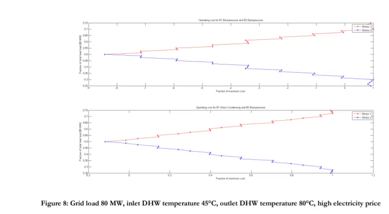
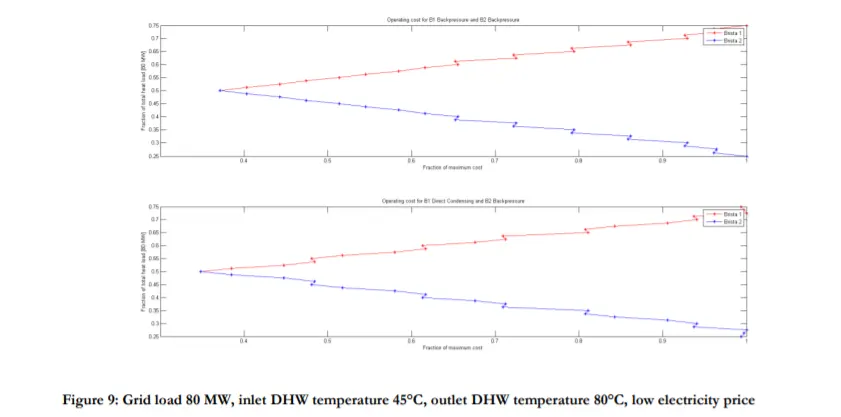
The figures clearly show that at a high electricity price, it is significantly more profitable to run both plants
in backpressure mode rather than running B1 in direct condensing mode. In either case, an approximately
50%-50% split between the two plants, i.e. B1 producing 40 MW and B2 producing 40 MW, is the most
cost-efficient allocation of heat production.
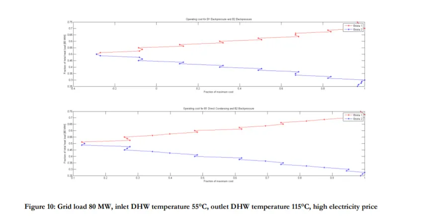
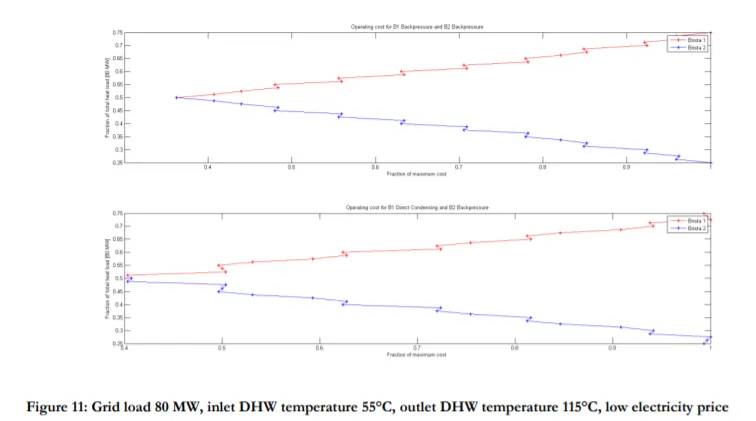
There seems to be no significant difference in heat allocation due to the higher DHW temperature, and
the same allocation as in the 80/45°C case is preferred. However, the potential profits at high electricity
prices are significantly lower. This is likely due to the higher DHW temperature requiring a higher exit
pressure from the low-pressure turbine stage, causing a lower pressure drop over the turbine. This reduces
the electricity production, which in turn reduces the amount of electricity available to sell.
% MJ211X Degree Project in Thermal Engineering, KTH 2012
% Thesis title: "Strategies for co-operated wood chip fired and municipal
% waste fired combined heat and power plants"
% Written by Alexander Taylor 860909-7491
% Version dated: 2012-05-29
% This program was written on assignment from Fortum Heat Scandinavia AB
% This is the main control program for simulating the combined operation of
% the Brista 1 and 2 plants. It requires the following modules in the same
% folder in order to run:
% B1_BP.m
% B1_DC.m
% B2_BP.m
% ComputeDHWFlow_BP.m
% ComputeEnthalpies_BP.m
% ComputeEnthalpies_BP_B2.m
% ComputeEnthalpies_DC.m
% ComputeFlueGas.m
% ComputePressures_BP.m
% ComputePressures_BP_B2.m
% ComputeTemperatures_BP.m
% ComputeTemperatures_BP_B2.m
% FindTurbineEfficiency.m
% FindTurbineEfficiency_B2.m
% XSteam.m
% The XSteam library is used with kind permission from www.x-eng.com
% This program computes the operating costs for the combined operation of
% the two plants at a user-defined grid load and user-defined range of
% electricity prices and plots the results.
clear all
close all
clc
% Set which operating modes should be included; BP = Backpressure, DC =
% Direct condensing, B1 = Brista 1, B2 = Brista 2
BP_B1 = 1;
BP_B2 = 1;
DC_B1 = 1;
% Main program to compute economics of plant operation
% Set range of electricity prices [kr/MWh] and step size. Make sure step
% size is an even multiple of the min/max price.
el_price_min =
el_price_max =
el_step = 100;
% Define max and min heat loads for both plants
heat_min_b1 = 40000;
heat_max_b1 = 105000;
heat_min_b2 = 20000;
heat_max_b2 = 60000;
% Define price and load vectors [kr/MWh]
el = el_price_min:el_step:el_price_max;
fuel_price_B1 = 226;
fuel_price_B2 = -122;
% Define other costs
% Operation & maintenance [kr/MWh]
op_maint =
% NOx related: Year-average nox production [mg/Nm3], cost [kr/kg]
average_nox =
cost_nox =
% Compute relevant combinations of b1 and b2 that fulfill the load
% requirement given min/max constraints. Make sure heat_step is an even
% multiple of heat_min and heat_max for both plants.
heat_step = 1000;
% Vectors of all possible values of heat production for b1 and b2 given an
% arbitrary step size
heat_b1 = heat_min_b1:heat_step:heat_max_b1;
heat_b2 = heat_min_b2:heat_step:heat_max_b2;
% Set goal value for heat production - the algorithm will compute all
% combinations of b1 and b2 that return this goal value. Make sure that the
% goal value is a multiple of the heat step size!
heat_goal =
totcost_BP_B1 = [];
totcost_BP_FG_B1 = [];
totcost_DC_B1 = [];
% Computes all possible combinations of b1 and b2 with the given heat step
% size that return the heat goal value. Returns these values as a 2xn
% matrix where column 1 is B1 output and column 2 is B2 output.
combinations = [];
kk = 1;
for ii = 1:length(heat_b1)
for jj = 1:length(heat_b2)
if (heat_b1(ii) + heat_b2(jj)) == heat_goal
combinations(kk,1) = heat_b1(ii);
combinations(kk,2) = heat_b2(jj);
kk = kk + 1;
end
end
end
disp(['Current heat load yields ' num2str(length(combinations)) ' possible
combinations of B1 and B2']);
disp('Running simulations, please wait...');
fprintf('\n');
costs_BP_B1 = zeros(length(combinations),length(el));
costs_BP_FG_B1 = zeros(length(combinations),length(el));
costs_DC_B1 = zeros(length(combinations),length(el));
costs_DC_FG_B1 = zeros(length(combinations),length(el));
costs_BP_B2 = zeros(length(combinations),length(el));
costs_BP_B2_tot = zeros(length(combinations),length(el));
costs_DC_B1_tot = zeros(length(combinations),length(el));
hours = zeros(2,length(el));
% Preallocate data vectors
B1_BP_data = zeros(length(combinations),5);
B1_BP_FG_data = zeros(length(combinations),5);
B1_DC_data = zeros(length(combinations),6);
B1_DC_FG_data = zeros(length(combinations),6);
B2_BP_data = zeros(length(combinations),5);
% Set relevant input data & constraints
t_dhw_in = 45;
t_dhw_out = 80;
mass_step = 1;
mass_start = 10;
% Compute power production, fuel flow, etc for each possible combination
for ii = 1:length(combinations)
% Dump data directly into data vectors
if BP_B1 == 1
B1_BP_data(ii,:) =
B1_BP(combinations(ii,1),0,mass_start,mass_step,t_dhw_in,t_dhw_out);
B1_BP_FG_data(ii,:) =
B1_BP(combinations(ii,1),1,mass_start,mass_step,t_dhw_in,t_dhw_out);
end
if DC_B1 == 1
B1_DC_data(ii,:) =
B1_DC(combinations(ii,1),0,mass_start,mass_step,t_dhw_in,t_dhw_out);
B1_DC_FG_data(ii,:) =
B1_DC(combinations(ii,1),1,mass_start,mass_step,t_dhw_in,t_dhw_out);
end
if BP_B2 == 1
B2_BP_data(ii,:) =
B2_BP(combinations(ii,2),mass_start,mass_step,t_dhw_in,t_dhw_out);
end
end
% Compute costs for each scenario
% Cost matrices will be constructed with each row corresponding to the
% total cost of one scenario and each column corresponding to the total
% cost of each item, i.e. electricity revenue, fuel costs, etc.
% Compute internal electricity consumption
internal_B1 =
internal_B2 =
for tt = 1:length(el)
% Compute total cost as fuel cost - electricity revenue + op/maint cost +
% nox cost + internal electricity consumption cost
if BP_B1 == 1
costs_BP_B1(:,tt) = B1_BP_data(:,3)*(fuel_price_B1/1000) +
B1_BP_data(:,1)*(-el(tt)/1000)...
+ B1_BP_data(:,2)*(op_maint/1000) +
B1_BP_data(:,5)*average_nox*(10^-6)*cost_nox*3600 ...
+ internal_B1*el(tt);
costs_BP_FG_B1(:,tt) = B1_BP_FG_data(:,3)*(fuel_price_B1/1000) +
B1_BP_FG_data(:,1)*...
(-el(tt)/1000) + B1_BP_FG_data(:,2)*(op_maint/1000) +
B1_BP_data(:,5)*average_nox*(10^-6)*cost_nox*3600 ...
+ internal_B1*el(tt);
end
if DC_B1 == 1
costs_DC_B1(:,tt) = B1_DC_data(:,4)*(fuel_price_B1/1000) +
B1_DC_data(:,3)*(op_maint/1000) + ...
B1_DC_data(:,6)*average_nox*(10^-6)*cost_nox*3600 +
internal_B1*el(tt);
costs_DC_FG_B1(:,tt) = B1_DC_FG_data(:,4)*(fuel_price_B1/1000) +
B1_DC_FG_data(:,3)*(op_maint/1000) ...
+ B1_DC_data(:,6)*average_nox*(10^-6)*cost_nox*3600 +
internal_B1*el(tt);
end
if BP_B2 == 1
costs_BP_B2(:,tt) = B2_BP_data(:,3)*(fuel_price_B2/1000) +
B2_BP_data(:,1)*(-el(tt)/1000)...
+ B2_BP_data(:,2)*(op_maint/1000) +
B2_BP_data(:,5)*average_nox*(10^-6)*cost_nox*3600 ...
+ internal_B2*el(tt);
end
% Compute total cost of each combination of operating modes
if BP_B1 && BP_B2 == 1
costs_BP_B2_tot(:,tt) = costs_BP_FG_B1(:,tt) + costs_BP_B2(:,tt);
end
if DC_B1 && BP_B2 == 1
costs_DC_B1_tot(:,tt) = costs_DC_FG_B1(:,tt) + costs_BP_B2(:,tt);
end
disp('Simulation complete!');
fprintf('\n');
% Convert load of both plants into fractions of 100%
fractions = combinations./heat_goal;
% Plotting
figure(tt)
subplot(2,1,1)
plot(costs_BP_B2_tot(:,tt),fractions(:,1),'-
*r',costs_BP_B2_tot(:,tt),fractions(:,2),'-*b')
ylabel(['Fraction of total heat load [' num2str(heat_goal/1000) ' MW]'])
xlabel('Total cost [kr/h]')
title(['Operating cost for B1 Backpressure and B2 Backpressure at p_el = '
num2str(el(tt)) ' kr/MWh']);
legend('Brista 1','Brista 2')
subplot(2,1,2)
plot(costs_DC_B1_tot(:,tt),fractions(:,1),'-
*r',costs_DC_B1_tot(:,tt),fractions(:,2),'-*b')
ylabel(['Fraction of total heat load [' num2str(heat_goal/1000) ' MW]'])
xlabel('Total cost [kr/h]')
title(['Operating cost for B1 Direct Condensing and B2 Backpressure at p_el
= ' num2str(el(tt)) ' kr/MWh']);
legend('Brista 1','Brista 2')
% Compute start/stop costs
cost_warm =
cost_cold =
revenue_BP = min(costs_BP_B2_tot(:,tt));
if revenue_BP <= 0
hours_warm = cost_warm/revenue_BP;
hours_cold = cost_cold/revenue_BP;
disp(['Number of hours revenue required to reach warm start cost: '
num2str(round(hours_warm))]);
disp(['Number of hours revenue required to reach cold start cost: '
num2str(round(hours_cold))]);
end
if revenue_BP >= 1
hours_warm = cost_warm/revenue_BP;
hours_cold = cost_cold/revenue_BP;
disp(['Number of hours loss required to reach warm start cost: '
num2str(round(hours_warm))]);
disp(['Number of hours loss required to reach cold start cost: '
num2str(round(hours_cold))]);
end
hours(1,tt) = hours_warm;
hours(2,tt) = hours_cold;
revenue(tt) = revenue_BP;
end
% Plotting
disp('Plotting results...');
fprintf('\n')
B1_BP.m
function [output] = B1_BP( Q_heat,FlueGasFlag,m,m_step,t_dhw_in,t_dhw_out )
% Set boiler power threshold [kW]
Q_boil_max = 122000;
% Set steam flow threshold [kg/s];
m_max = 50;
% Set turbine power thresholds
P_T_min = 4000;
P_T_max = 43000;
% Preallocate warning flags
flag = 0;
% Preallocate heating variables to make while-loop argument valid
Q_cond1 = 0;
Q_cond2 = 0;
Q_fg = 0;
gasflow = 0;
while (Q_cond1 + Q_cond2 + Q_fg) <= Q_heat
% Total steam load through boiler
m = m + m_step;
% Ensure that steam load does not exceed threshold
if m >= m_max
break
end
% Incoming and outgoing DHW temperature, pressure
p_dhw = 6;
dt = t_dhw_out - t_dhw_in;
% Known/assumed efficiencies
n_boil =
n_is_hp =
n_is_lp =
n_t = FindTurbineEfficiency(m,dt);
n_cond =
% Compute pressures, temperatures and enthalpies. These vectors have the
% following structures:
% Pressures: [p1 p1a p1b p1c p2 p2a p2b p3 p6 p7]
% Temperatures: [t1 t1aa t1ab t7 tint]
% Enthalpies: [h1 h1a h1b h1c h1aa h1ab h2 h2a h2b h3 h4a h4b h6 h7]
Pressures = ComputePressures_BP(m,dt);
Temperatures = ComputeTemperatures_BP(m,dt);
Enthalpies = ComputeEnthalpies_BP(Temperatures,Pressures,n_is_hp,n_is_lp);
% Compute DHW data - mass flow, intermediate temperature, enthalpies and
% heat load
h_dhw_in = XSteam('h_pT',p_dhw,t_dhw_in);
h_dhw_out = XSteam('h_pT',p_dhw,t_dhw_out);
m_dhw = ComputeDHWFlow_BP(m,dt);
% Compute boiler load
Q_boil = (1/n_cond)*m*(Enthalpies(1) - Enthalpies(15));
Q_fuel = Q_boil/n_boil;
% Ensure that boiler power does not exceed threshold!
if Q_boil >= Q_boil_max
break
end
% Compute combustion data
% Convert LHV from MJ/kg to kJ/kg
HHV =
fuelflow = Q_fuel/HHV;
% Flue gas condensation computations
if FlueGasFlag == 1
C =
H =
O =
N =
S =
moist =
gasflow = ComputeFlueGas( C,H,N,O,S,moist);
gasflow = gasflow*fuelflow;
% Based on maximum flue gas condensation heat
% output of 30 MW @ 50kg/s steam load
dh_gas = 591.1439;
Q_fg = gasflow*dh_gas;
m_dhw_fg = (gasflow*dh_gas)/(h_dhw_out - h_dhw_in);
% Total dhw flow is the sum of the boiler load flow and the flue gas
% contribution
m_dhw_tot = m_dhw + m_dhw_fg;
else
m_dhw_tot = m_dhw;
end
% Compute intermediate dhw data
t_dhw_int = XSteam('Tsat_p',Pressures(8)) - 1;
h_dhw_int = XSteam('h_pT',p_dhw,t_dhw_int);
% Construct linear equation system. Structure depends on whether stream 2a
% has to be closed or not (i.e. if p2b > p2a).
if Enthalpies(8) > 0
PrintFlag = 0;
A = [(Enthalpies(2)-Enthalpies(5)) 0 0 0 0 0 0;
(Enthalpies(5)-Enthalpies(6)) (Enthalpies(3)-Enthalpies(6)) 0 0 0 0
0;
1 1 1 1 0 0 0;
0 0 0 -1 1 1 1;
0 0 0 0 0 (Enthalpies(9)-Enthalpies(11)) 0;
0 0 0 0 0 0 (Enthalpies(10)-Enthalpies(12));
];
b = [m*(Enthalpies(15) - Enthalpies(14));
m*(Enthalpies(14) - Enthalpies(13));
m;
0;
(1/n_cond)*m_dhw*(h_dhw_out - h_dhw_int);
(1/n_cond)*m_dhw*(h_dhw_int - h_dhw_in);
];
else
PrintFlag = 1;
A = [(Enthalpies(2)-Enthalpies(5)) 0 0 0 0 0;
(Enthalpies(5)-Enthalpies(6)) (Enthalpies(3)-Enthalpies(6)) 0 0 0
0;
1 1 1 1 0 0;
0 0 0 -1 1 1;
Enthalpies(6) Enthalpies(6) Enthalpies(4) 0 Enthalpies(11)
Enthalpies(12);
0 0 0 0 (Enthalpies(9)-Enthalpies(11)) 0;
0 0 0 0 0 (Enthalpies(10)-Enthalpies(12));
];
b = [m*(Enthalpies(15) - Enthalpies(14));
m*(Enthalpies(14) - Enthalpies(13));
m;
0;
m*Enthalpies(13);
(1/n_cond)*m_dhw*(h_dhw_out - h_dhw_int);
(1/n_cond)*m_dhw*(h_dhw_int - h_dhw_in);
];
end
% Solve linear equation system
sol = A\b;
% Compute power output of turbines
P_HP = (m*(Enthalpies(1) - Enthalpies(2)) + (m-sol(1))*(Enthalpies(2) -
Enthalpies(3))...
+ (m - sol(1) - sol(2))*(Enthalpies(3) - Enthalpies(4)) + (m - sol(1) -
sol(2) ...
- sol(3))*(Enthalpies(4) - Enthalpies(7)))*n_t;
% LP turbine expansion line depends on whether steam extraction at point 2a
% is performed or not, therefore the power equation must change accordingly
if Enthalpies(8) > 0
P_LP = (sol(4)*(Enthalpies(7) - Enthalpies(8)) + (sol(4) -
sol(5))*(Enthalpies(8) - ...
Enthalpies(9)) + (sol(4) - sol(5) - sol(6))*(Enthalpies(9) -
Enthalpies(10)))*n_t;
Q_cond1 = n_cond*sol(6)*(Enthalpies(9)-Enthalpies(11));
Q_cond2 = n_cond*sol(7)*(Enthalpies(10)-Enthalpies(12));
else
P_LP = (sol(4)*(Enthalpies(7) - Enthalpies(9)) + (sol(4) -
sol(5))*(Enthalpies(9) - ...
Enthalpies(10)))*n_t;
Q_cond1 = n_cond*sol(5)*(Enthalpies(9)-Enthalpies(11));
Q_cond2 = n_cond*sol(6)*(Enthalpies(10)-Enthalpies(12));
end
end
% Output returned as vector with [Electrical power output, thermal power
% output, fuel heat input, fuel mass flow]
% Check all threholds!
if (P_HP+P_LP) > P_T_max
disp('WARNING: Turbine power exceeds maximum value!')
flag = 1;
end
if (P_HP+P_LP) < P_T_min
disp('WARNING: Turbine power lower than minimum value!')
flag = 1;
end
if Q_boil > Q_boil_max
disp('WARNING: Boiler power exceeded threshold!')
flag = 1;
end
if m > m_max
disp('WARNING: Steam flow exceeded threshold!')
flag = 1;
end
if flag == 0
disp('Simulation completed with no errors!')
fprintf('\n')
else
disp('There were one or more warnings during the simulation.')
fprintf('\n')
end
output = [(P_HP+P_LP) (Q_cond1 + Q_cond2 + Q_fg) Q_fuel fuelflow gasflow];
end